General Context-Aware Data Matching and Merging Framework
Slavko Žitnik, Lovro Šubelj, Dejan Lavbič, Olegas Vasilecas and Marko Bajec. 2013. General Context-Aware Data Matching and Merging Framework, Informatica (INFOR), 24(1), pp. 119 - 152.
Abstract
Due to numerous public information sources and services, many methods to combine heterogeneous data were proposed recently. However, general end-to-end solutions are still rare, especially systems taking into account different context dimensions. Therefore, the techniques often prove insufficient or are limited to a certain domain. In this paper we briefly review and rigorously evaluate a general framework for data matching and merging. The framework employs collective entity resolution and redundancy elimination using three dimensions of context types. In order to achieve domain independent results, data is enriched with semantics and trust. However, the main contribution of the paper is evaluation on five public domain-incompatible datasets. Furthermore, we introduce additional attribute, relationship, semantic and trust metrics, which allow complete framework management. Besides overall results improvement within the framework, metrics could be of independent interest.
Keywords
Entity resolution, redundancy elimination, semantic elevation, trust, ontologies
1 Introduction
Heterogeneous data matching and merging is due to increasing amount of linked and open (on-line) data sources rapidly becoming a common need in various fields. Different scenarios demand for analyzing heterogeneous datasets collectively, enriching data with some on-line data source or reducing redundancy among datasets by merging them into one. Literature provides several state-of-the-art approaches for matching and merging, although there is a lack of general solutions combining different dimensions arising during the matching and merging execution. We propose and evaluate a general and complete solution that allows a joint control over these dimensions.
Data sources commonly include not only network data, but also data with semantics. Thus a state-of-the-art solution should employ semantically elevated algorithms (i.e. algorithms that can process data with semantics according to an ontology), to fully exploit the data at hand. However, due to a vast diversity of data sources, an adequate data architecture also employed. In particular, the architecture should support all types and formats of data, and provide appropriate data for each algorithm. As algorithms favor different representations and levels of semantics behind the data, architecture should be structured appropriately.
Due to different origin of (heterogeneous) data sources, the trustworthiness (or accuracy) of their data can often be questionable. Specially, when many such datasets are merged, the results are likely to be inexact. A common approach for dealing with data sources that provide untrustworthy or conflicting statements, is the use of trust management systems and techniques. Thus matching and merging should be advanced to a trust-aware level, to jointly optimize trustworthiness of data and accuracy of matching or merging. Such collective optimization can significantly improve over other approaches.
The paper proposes and demonstrates a general framework for matching and merging execution. An adequate data architecture enables either pure related data, in the form of networks, or data with semantics, in the form of ontologies. Different datasets are merged using collective entity resolution and redundancy elimination algorithms, enhanced with trust management techniques. Algorithms are managed through the use of different contexts that characterize each particular execution, and can be used to jointly control various dimensions of variability of matching and merging execution. Proposed framework is also fully implemented and evaluated against real-world datasets.
The rest of the paper is structured as follows. The following section gives a brief overview of the related work, focusing mainly on trust-aware matching and merging. Next, section 3, presents employed data architecture and discusses semantic elevation of the proposition. Section 4 formalizes the notion of trust and introduces the proposed trust management techniques. General framework, and accompanying algorithms, for matching and merging are presented in section 5. Experimental demonstration of the proposed framework is shown in section 6, and further discussed in section 7. Section 8 concludes the paper.
3 Data architecture
An adequate data architecture is of vital importance for efficient matching and merging. Key issues arising are as follows:
- architecture should allow for data from heterogeneous sources, commonly in various formats,
- semantical component of data should be addressed properly and
- architecture should also deal with (partially) missing and uncertain data.
To achieve superior performance, we propose a three level architecture (see Figure 3.3). Standard network data representation on the bottom level (data level) is enriched with semantics (semantic level) and thus elevated towards the topmost real world level (abstract level). Datasets on data level are represented with networks, when the semantics are employed through the use of ontologies.
Every dataset is (preferably) represented on data and semantic level. Although both describe the same set of entities on abstract level, the representation on each level is independent from others. This separation resides from the fact that different algorithms of matching and merging execution privilege different representations of data - either pure related or semantically elevated representation. Separation thus results in more accurate and efficient matching and merging, moreover, representations can complement each other in order to boost the performance.
The following section gives a brief introduction to networks, used for data level representation. Section 3.2 describes ontologies and semantic elevation of data level (i.e. semantic level). Proposed data architecture is formalized and further discussed in Section 3.3.
3.1 Representation with networks
Most natural representation of any related data are networks (Newman 2010). They are based upon mathematical objects called graphs. Informally speaking, graph consists of a collection of points, called vertices, and links between these points, called edges (see Figure 3.1).
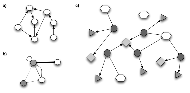
Figure 3.1: (a) directed graph; (b) labeled undirected multigraph (labels are represented graphically); (c) network representing a group of related restaurants (circles correspond to restaurants, hexagons to their types, triangles to different phone numbers, while squares represent respective cities).
Let \(V_N\), \(E_N\) be a set of vertices, edges for some graph \(N\) respectively. We define graph \(N\) as \(N=(V_N,E_N)\) where
\[\begin{equation} V_N = \{v_1, v_2 \dots v_n\} \tag{3.1} \end{equation}\] \[\begin{equation} E_N \subseteq \{\{v_i, v_j\}|\mbox { } v_i, v_j \in V_N \wedge i<j \} \tag{3.2} \end{equation}\]Edges are sets of vertices, hence they are not directed (undirected graph). In the case of directed graphs Equation (3.2) rewrites to
\[\begin{equation} E_N \subseteq \{(v_i, v_j)|\mbox { } v_i, v_j \in V_N \wedge i\neq j\} \tag{3.3} \end{equation}\]where \((v_i,v_j)\) is an edge from \(v_i\) to \(v_j\). The definition can be further generalized by allowing multiple edges between two vertices and loops (edges that connect vertices with themselves). Such graphs are called multigraphs (see Figure 3.1 b).
In practical applications we commonly strive to store some additional information along with the vertices and edges. Formally, we define labels or weights for each node and edge in the graph – they represent a set of properties that can also be described using two attribute functions
\[\begin{equation} A_{V_N}: V_N\rightarrow\Sigma_1^{V_N}\times\Sigma_2^{V_N}\times\dots \tag{3.4} \end{equation}\] \[\begin{equation} A_{E_N}: E_N\rightarrow\Sigma_1^{E_N}\times\Sigma_2^{E_N}\times\dots \tag{3.5} \end{equation}\]\(A_N=(A_{V_N}, A_{E_N})\), where \(\Sigma_i^{V_G}\), \(\Sigma_i^{E_G}\) are sets of all possible vertex, edge attribute values respectively.
Networks are most commonly seen as labeled, or weighted, multigraphs with both directed and undirected edges (see Figure 3.1 c). Vertices of a network represent some entities, and edges represent related data between them. A (related) dataset, represented with a network on the data level, is thus defined as \((N,A_N)\).
3.2 Semantic elevation using ontologies
Ontologies are formal definitions of classes, related data, functions and other objects. An ontology is an explicit specification of conceptualization (Gruber 1993), which is is an abstract view of the knowledge we wish to represent. It can be defined as a network of entities, restricted and annotated with a set of axioms. Let \(E_O\), \(A_O\) be the sets of entities, axioms for some ontology \(O\) respectively. We propose a dataset representation with an ontology on semantic level (an example in Figure 3.2 as \(O=(E_O,A_O)\) where
\[\begin{equation} E_O \subseteq E^C\cup E^I\cup E^R\cup E^A \tag{3.6} \end{equation}\] \[\begin{equation} A_O \subseteq \{a|\mbox{ }E_O^a\subseteq E_O\wedge a\mbox{ axiom on }E_O^a\} \tag{3.7} \end{equation}\]Entities \(E_O\) consist of classes \(E^C\) (concepts), individuals \(E^I\) (instances), related data \(E^R\) (among classes and individuals) and attributes \(E^A\) (properties of classes); and axioms \(A_O\) are assertions (over entities) in a logical form that together comprise the overall theory described by ontology \(O\).
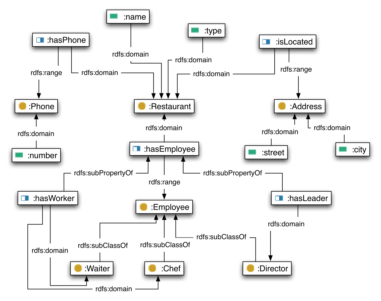
Figure 3.2: A possible ontology over Restaurants dataset (description in Section 6.1). Classes are represented by circles, related data by half-white rectangles and attributes by full-colour rectangles. Key concepts of the ontology are Restaurant, Address, Phone and Employee.
This paper focuses on ontologies based on descriptive logic that, besides assigning meaning to axioms, enable also reasoning capabilities (Horrocks and Sattler 2001). The latter can be used to compute consequences of the previously made assumptions (queries), or to discover non-intended consequences and inconsistencies within the ontology.
One of the most prominent applications of ontologies is in the domain of semantic interoperability (among heterogeneous software systems). While pure semantics concerns the study of meanings, we define semantic elevation as a process to achieve semantic interoperability which be considered as a subset of information integration.
Thus one of the key aspects of semantic elevation is to derive a common representation of classes, individuals, related data and attributes within some ontology. We employ a concept of knowledge chunks (Castano, Ferrara, and Montanelli 2010), where each entity is represented with its name, set of semantically related data, attributes and identifiers. All of the data about a certain entity is thus transformed into attribute-value format, with an identifier of the data source of origin appended to each value. Exact description of the transformation between networked data and knowledge chunks is not given, although it is very similar to the definition of inferred axioms in Equation (3.12), section 3.3. Knowledge chunks, denoted \(k \in K\), thus provide a (common) synthetic representation of an ontology that is used during the matching and merging execution. For more details on knowledge chunks, and their construction from a RDF(S)1 repository or an OWL2, see (Castano, Ferrara, and Montanelli 2010; Castano, Ferrara, and Montanelli 2009).
3.3 Three level architecture
As previously stated, every dataset is (independently) represented on three levels – data, semantic and abstract level (see Figure 3.3). Bottommost data level holds data in a pure related format (i.e. networks), mainly to facilitate state-of-the-art related data algorithms for matching. Next level, semantic level, enriches data with semantics (i.e. ontologies), to further enhance matching and to promote semantic merging execution. Data on both levels represent entities of topmost abstract level, which serves merely as an abstract (artificial) representation of all the entities, used during matching and merging execution.
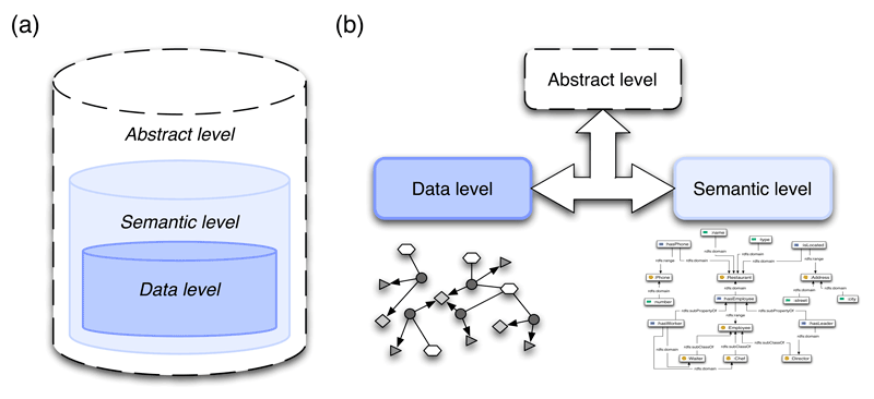
Figure 3.3: (a) information-based view of the data architecture; (b) data-based view of the data architecture
The information captured by data level is a subset of that of semantic level. Similarly, the information captured by semantic level is a subset of that of abstract level. This information-based view of the architecture is seen in Figure 3.3 a). However, representation on each level is completely independent from the others, due to absolute separation of data. This provides an alternative data-based view, seen in Figure 3.3 b).
To manage data and semantic level independently (or jointly), a mapping between the levels is required. In practice, data source could provide datasets on both, data and semantic level. The mapping is in that case trivial (i.e. given). However, more commonly, data source would only provide datasets on one of the levels, and the other has to be inferred.
Let \((N, A_N)\) be a dataset, represented as a network on data level. Without loss for generality, we assume that \(N\) is an undirected network. Inferred ontology \((\tilde{E}_{\tilde{O}}, \tilde{A}_{\tilde{O}})\) on semantic level is defined with
\[\begin{equation} \tilde{E}_C = \{vertex, edge\} \tag{3.8} \end{equation}\] \[\begin{equation} \tilde{E}_I = V_N\cup E_N \tag{3.9} \end{equation}\] \[\begin{equation} \tilde{E}_R = \{isOf, isIn\} \tag{3.10} \end{equation}\] \[\begin{equation} \tilde{E}_A = \{A_{V_N}, A_{E_N}\} \tag{3.11} \end{equation}\]and
\[\begin{equation} \begin{split} \tilde{A}_{\tilde{O}} = & \text{ } \{v \text{ isOf vertex } | \text{ } v \in V_N\} \\ & \cup \text{ } \{e \text{ isOf edge } | \text{ } e \in E_N\} \\ & \cup \text{ } \{v \text{ isIn } e \text{ } | \text{ } v \in V_N \wedge e \in E_N \wedge v \in e\} \\ & \cup \text{ } \{v.A_{V_N} = a \text{ } | \text{ } v \in V_N\wedge A_{V_N}(v) = a\} \\ & \cup \text{ } \{e.A_{E_N} = a \text{ } | \text{ } e \in E_N \wedge A_{E_N}(e) = a\} \end{split} \tag{3.12} \end{equation}\]We denote \(\mathcal{I}_N: (N,A_N)\mapsto (\tilde{E}_{\tilde{O}},\tilde{A}_{\tilde{O}})\). One can easily see that \(\mathcal{I}_N^{-1}\circ \mathcal{I}_N\) is an identity (transformation preserves all the information).
On the other hand, given a dataset \((E_O,A_O)\), represented with an ontology on semantic level, inferred (undirected) network \((\tilde{N},\tilde{A}_{\tilde{N}})\) on data level is defined with
\[\begin{equation} \tilde{V}_{\tilde{N}} = E_O\cap E^I \tag{3.13} \end{equation}\] \[\begin{equation} \tilde{E}_{\tilde{N}} = \{E_O^a\cap E^I|\mbox{ }a\in A_O\wedge E_O^a\subseteq E_O\} \tag{3.14} \end{equation}\]and
\[\begin{equation} \tilde{A}_{\tilde{V}_{\tilde{N}}}: \tilde{V}_{\tilde{N}}\rightarrow E^C\times E^A \tag{3.15} \end{equation}\] \[\begin{equation} \tilde{A}_{\tilde{E}_{\tilde{N}}}: \tilde{E}_{\tilde{N}}\rightarrow E^R \tag{3.16} \end{equation}\]Instances of ontology are represented with the vertices of the network, and axioms with its edges. Classes and related data are, together with the attributes, expressed through vertex, edge attribute functions.
We denote \(\mathcal{I}_O: (E_O,A_O)\mapsto (\tilde{N},\tilde{A}_{\tilde{N}})\). Transformation \(\mathcal{I}_O\) discards purely semantic information (e.g. related data between classes), as it cannot be represented on the data level. Thus \(\mathcal{I}_O\) cannot be inverted as \(\mathcal{I}_N\). However, all the data, and data related information, is preserved (e.g. individuals, classes and related data among individuals).
Due to limitations of networks, only axioms, relating at most two individuals in \(E_O\), can be represented with the set of edges \(\tilde{E}_{\tilde{N}}\) (see Equation (3.14)). When this is not sufficient, hypernetworks (or hypergraphs3) should be employed instead. Nevertheless, networks should suffice in most cases.
One more issue has to be stressed. Although \(\mathcal{I}_N\) and \(\mathcal{I}_O\) give a “common” representation of every dataset, the transformations are completely different. For instance, presume \((N,A_N)\) and \((E_O,A_O)\) are (given) representations of the same dataset. Then \(\mathcal{I}_N(N,A_N)\neq (E_O,A_O)\) and \(\mathcal{I}_O(E_O,A_O)\neq (N,A_N)\) in general – inferred ontology, network does not equal given ontology, network respectively. The former non-equation resides in the fact that network \((N,A_N)\) contains no knowledge of the (pure) semantics within ontology \((E_O,A_O)\); and the latter resides in the fact that \(\mathcal{I}_O\) has no information of the exact representation used for \((N,A_N)\). Still, transformations \(\mathcal{I}_N\) and \(\mathcal{I}_O\) can be used to manage data on a common basis.
Last, we discuss three key issues regarding an adequate data architecture, presented in Section 3. Firstly, due to variety of different data formats, a mutual representation must be employed. As the data on both data and semantic level is represented in the form of knowledge chunks (see Section 3.2), every piece of data is stored in exactly the same way. This allows for common algorithms of matching and merging and makes the data easily manageable.
Furthermore, introduction of knowledge chunks naturally deals also with missing data. As each chunk is actually a set of attribute-value pairs, missing data only results in smaller chunks. Alternatively, missing data could be randomly inputted from the rest and treated as extremely uncertain or mistrustful (see Section 4).
Secondly, semantical component of data should be addressed properly. Proposed architecture allows simple (related) data and also semantically enriched data. Hence no information is discarded. Moreover, appropriate transformations make all data accessible on both data and semantic level, providing for specific needs of each algorithm.
Thirdly, architecture should deal with (partially) missing and uncertain or mistrustful data, which is thoroughly discussed in the following section.
4 Trust and trust management
When merging data from different sources, these are often of different origin and thus their trustworthiness (or accuracy) can be questionable. For instance, personal data of participants in a traffic accident is usually more accurate in the police record of the accident, then inside participants’ social network profiles. Nevertheless, an attribute from less trusted data source can still be more accurate than an attribute from more trusted one – a related status (e.g. single or married) in the record may be outdated, while such type of information is inside the social network profiles quite often up-to-date.
A complete solution for matching and merging execution should address such problems as well. A common approach for dealing with data sources that provide untrustworthy or conflicting statements, is the use of trust management (systems). These are, alongside the concept of trust, both further discussed in sections 4.1 and 4.2.
4.1 Definition of trust
Trust is a complex psychological-sociological phenomenon. Despite of, people use term trust in everyday life widely, and with very different meanings. Most common definition states that trust is an assured reliance on the character, ability, strength, or truth of someone or something.
In the context of computer networks, trust is modeled as a related data between entities. Formally, we define a trust related data as
\[\begin{equation} \omega_E: E\times E\rightarrow \Sigma^E \tag{4.1} \end{equation}\]where \(E\) is a set of entities and \(\Sigma^E\) a set of all possible, numerical or descriptive, trust values. \(\omega_E\) thus represents one entity’s attitude towards another and is used to model trust(worthiness) of all entities in \(E\). To this end, different trust modeling methodologies and systems can be employed, from qualitative to quantitative (e.g. (Nagy, Vargas-Vera, and Motta 2008; Richardson, Agrawal, and Domingos 2003; Trček 2009)).
We introduce trust on three different levels. First, we define trust on the level of data source, in order to represent trustworthiness of the source in general. Let \(S\) be the set of all data sources. Their trust is defined as \(T_S: S\rightarrow [0,1]\), where higher values of \(T_S\) represent more trustworthy source.
Second, we define trust on the level of attributes (or semantically related data) within the knowledge chunks. The trust in attributes is naturally dependent on the data source of origin, and is defined as \(T_{A_s}: A_s\rightarrow [0,1]\), where \(A_s\) is the set of attributes for data source \(s\in S\). As before, higher values of \(T_{A_s}\) represent more trustworthy attribute.
Last, we define trust on the level of knowledge chunks. Despite the trustworthiness of data source and attributes within some knowledge chunk, its data can be (semantically) corrupted, missing or otherwise unreliable. This information is captured using trustworthiness of knowledge chunks, and again defined as \(T_{K}: K\rightarrow [0,1]\), where \(K\) is a set of all knowledge chunks. Although the trust related data (see Equation (4.1)), needed for the evaluation of trustworthiness of data sources and attributes, are (mainly) defined by the user, computation of trust in knowledge chunks can be fully automated using proper evaluation function (see Section 4.2).
Three levels of trust provide high flexibility during matching and merging. For instance, attributes from more trusted data sources are generally favored over those from less trusted ones. However, by properly assigning trust in attributes, certain attributes from else less trusted data sources can prevail. Moreover, trust in knowledge chunks can also assist in revealing corrupted, and thus questionable, chunks that should be excluded from further execution.
Finally, we define trust in some particular value within a knowledge chunk, denoted trust value \(T\). This is the value in fact used during merging and matching execution and is computed from corresponding trusts on all three levels. In general, \(T\) can be an arbitrary function of \(T_S\), \(T_{A_s}\) and \(T_K\). Assuming independence, we calculate trust value by concatenating corresponding trusts
\[\begin{equation} T = T_{S} \circ T_{A_s} \circ T_{K} \tag{4.2} \end{equation}\]Concatenation function \(\circ\) could be a simple multiplication or some fuzzy logic operation (trusts should in this case be defined as fuzzy sets).
4.2 Trust management
During merging and matching execution, trust values are computed using trust management algorithm based on (Richardson, Agrawal, and Domingos 2003). We begin by assigning trust values \(T_S\), \(T_{A_s}\) for each data source, attribute respectively (we actually assign trust related data). Commonly, only a subset of values must necessarily be assigned, as others can be inferred or estimated from the first. Next, trust values for each knowledge chunk are not defined by the user, but are calculated using the chunk evaluation function \(f_{eval}\) (i.e. \(T_K=f_{eval}\)).
An example of such function is a density of inconsistencies within some knowledge chunk. For instance, when attributes Birth and Age of some particular knowledge chunk mismatch, this can be seen as an inconsistency. However, one must also consider the trust of the corresponding attributes (and data sources), as only inconsistencies among trustworthy attributes should be considered. Formally, density of inconsistencies is defined as
\[\begin{equation} f_{eval}(k) = \frac{\hat{N}_{inc}(k)-N_{inc}(k)}{\hat{N}_{inc}(k)}, \tag{4.3} \end{equation}\]where \(k\) is a knowledge chunk, \(k\in K\), \(N_{inc}(k)\) the number of inconsistencies within \(k\) and \(\hat{N}_{inc}(k)\) the number of all possible inconsistencies.
Finally, after all individual trusts \(T_S\), \(T_{A_s}\) and \(T_K\) have been assigned, trust values \(T\) are computed using equation (4.2). When merging takes place and two or more data sources (or knowledge chunks) provide conflicting attribute values, corresponding to the same (resolved) entity, trust values \(T\) are used to determine actual attribute value in the resulting data source (or knowledge chunk). For further discussion on trust management during matching and merging see Section 5.
5 Matching and merging data sources
Merging data from heterogeneous sources can be seen as a two-step process. The first step resolves the real world entities of abstract level, described by the data on lower levels, and constructs a mapping between the levels. This mapping is used in the second step that actually merges the datasets at hand. We denote these subsequent steps as entity resolution (i.e. matching) and redundancy elimination (i.e. merging).
Matching and merging is employed in various scenarios. As the specific needs of each scenario vary, different dimensions of variability characterize every matching and merging execution. These dimensions are managed through the use of contexts (Castano, Ferrara, and Montanelli 2010; Lapouchnian and Mylopoulos 2009). Contexts allow a formal definition of specific needs arising in diverse scenarios and a joint control over various dimensions of matching and merging execution.
The following section discusses the notion of contexts more thoroughly and introduces different types of contexts used. Next, sections 5.2 and 5.3 describe employed entity resolution and redundancy elimination algorithms respectively. The general framework for matching and merging is presented and formalized in Section 5.4, and discussed in Section 7.
5.1 Contexts
Every matching and merging execution is characterized by different dimensions of variability of the data, and mappings between. Contexts are a formal representation of all possible operations in these dimensions, providing for specific needs of each scenario. Every execution is thus characterized with the contexts it defines (see Figure 5.1), and can be managed and controlled through their use.
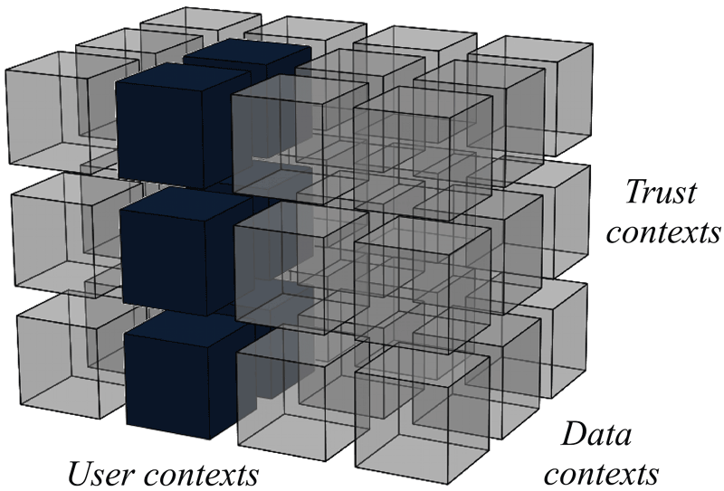
Figure 5.1: Characterization of merging and matching execution defining one context in user dimension, two contexts in data dimension and all contexts in trust dimension
The idea of contexts originates in the field of requirements engineering, where it has been applied to model domain variability (Lapouchnian and Mylopoulos 2009). It has just recently been proposed to model also variability of the matching execution (Castano, Ferrara, and Montanelli 2010). Our work goes one step further as it introduces contexts, not bounded only to user or scenario specific dimensions, but also data related and trust contexts.
Formally, we define a context \(C\) as
\[\begin{equation} C: D \rightarrow \{true, false\}, \tag{5.1} \end{equation}\]where \(D\) can be any simple or composite domain. A context simply limits all possible values, attributes, related data, knowledge chunks, datasets, sources or other, that are considered in different parts of matching and merging execution. Despite its simple definition, a context can be a complex function. It is defined on any of the architecture levels, preferably on all. Let \(C_A\), \(C_S\) and \(C_D\) represent the same context on abstract, semantic and data level respectively. The joint context is defined as
\[\begin{equation} C_J = C_A \wedge C_S \wedge C_D \tag{5.2} \end{equation}\]In the case of missing data (or contexts), only appropriate contexts are considered. Alternatively, contexts could be defined as fuzzy sets, to address also the noisiness of data. In that case, a fuzzy \(\mathsf{AND}\) operation should be used to derive joint context \(C_J\).
We distinguish between three types of contexts due to different dimensions characterized (see Figure 5.1).
- User or scenario specific contexts are used mainly to limit the data and control the execution. This type coincides with dimensions identified in (Castano, Ferrara, and Montanelli 2010). An example of user context is a simple selection or projection of the data.
- Data related contexts arise from dealing with related or semantic data, and various formats of data. Missing or corrupted data can also be managed through the use of these contexts.
- Trust and data uncertainty contexts provide for an adequate trust management and efficient security assurance between and during different phases of execution. An example of trust context is a definition of required level of trustworthiness of data or sources.
Detailed description of each context is out of scope of this paper. For more details on (user) contexts see (Castano, Ferrara, and Montanelli 2010).
5.2 Entity resolution
First step of matching and merging execution is to resolve the real world entities on abstract level, described by the data on lower levels. Thus a mapping between the levels (entities) is constructed and used in consequent merging execution. Recent literature proposes several state-of-the-art approaches for entity resolution (e.g. (Ananthakrishna, Chaudhuri, and Ganti 2002; Bhattacharya and Getoor 2004; Bhattacharya and Getoor 2007; Dong, Halevy, and Madhavan 2005; Kalashnikov and Mehrotra 2006). A naive approach is a simple pairwise comparison of attribute values among different entities. Although, such an approach could already be sufficient for flat data, this is not the case for network data, as the approach completely discards related data between the entities. For instance, when two entities are related to similar entities, they are more likely to represent the same entity. However, only the attributes of the related entities are compared, thus the approach still discards the information if related entities resolve to the same entities – entities are even more likely to represent the same entities when their related entities resolve to, not only similar, but the same entities. An approach that uses this information, and thus resolves entities altogether (in a collective fashion), is denoted collective (related) entity resolution algorithm.
We employ a state-of-the-art (collective) related data clustering algorithm proposed in (Bhattacharya and Getoor 2007). To further enhance the performance, algorithm is semantically elevated and adapted to allow for proper and efficient trust management.
The algorithm 5.1 is actually a greedy agglomerative clustering. Entities (on lower levels) are represented as a group of clusters \(C\), where each cluster represents a set of entities that resolve to the same entity on abstract level. At the beginning, each (lower level) entity resides in a separate cluster. Then, at each step, the algorithm merges two clusters in \(C\) that are most likely to represent the same entity (most similar clusters). When the algorithm unfolds, \(C\) holds a mapping between the entities on each level (i.e. maps entities on lower levels through the entities on abstract level).
During the algorithm, similarity of clusters is computed using a joint similarity measure (see Equation (5.9)), combining attribute, related data and semantic similarity. First is a basic pairwise comparison of attribute values, second introduces related information into the computation of similarity (in a collective fashion), while third represents semantic elevation of the algorithm.
Let \(c_i, c_j\in C\) be two clusters of entities. Using knowledge chunk representation, attribute cluster similarity is defined as
\[\begin{equation} sim_A(c_i, c_j) = \sum_{k_{i,j} \in c_{i,j} \wedge a \in k_{i,j}} trust(k_i.a, k_j.a) sim_A(k_i.a, k_j.a), \tag{5.3} \end{equation}\]where \(k_{i,j}\in K\) are knowledge chunks, \(a\in A_s\) is an attribute and \(sim_A(k_i.a, k_j.a)\) similarity between two attribute values. (Attribute) similarity between two clusters is thus defined as a weighted sum of similarities between each pair of values in each knowledge chunk. Weights are assigned due to trustworthiness of values – trust in values \(k_i.a\) and \(k_j.a\) is computed using
\[\begin{equation} trust(k_i.a, k_j.a) = \min\{T(k_i.a), T(k_j.a)\} \tag{5.4} \end{equation}\]Hence, when even one of the values is uncertain or mistrustful, similarity is penalized appropriately, to prevent matching based on (likely) incorrect information.
For computation of similarity between actual attribute values \(sim_A(k_i.a, k_j.a)\) (see Equation (5.3)), different measures have been proposed. Levenshtein distance (Levenshtein 1966) measures edit distance between two strings – number of insertions, deletions and replacements that traverse one string into the other. Another class of similarity measures are TF-IDF4-based measures (e.g. Cos TF-IDF and Soft TF-IDF (Cohen, Ravikumar, and Fienberg 2003; Moreau, Yvon, and CappÈ 2008)). They treat attribute values as a bag of words, thus the order of words in the attribute has no impact on the similarity. Other attribute measures are also Jaro (Jaro 1989) and Jaro-Winkler (Winkler 1990) that count number of matching characters between the attributes.
Different similarity measures prefer different types of attributes. TF-IDF-based measures work best with longer strings (e.g. descriptions), when other prefer shorter strings (e.g. names). For numerical attributes, an alternative measure has to be employed (e.g. simple evaluation, followed by a numerical comparison). Therefore, when computing attribute similarity for a pair of clusters, different attribute measures are used with different attributes (see Equation (5.3)).
Using data level representation, we define a for vertex \(v\in V_N\) as
\[\begin{equation} nbr(v) = \{v_n|\mbox{ }v_n\in V_N\wedge \{v, v_n\}\in E_N\} \tag{5.5} \end{equation}\]and cluster \(c\in C\) as
\[\begin{equation} nbr(c) = \{c_n|\mbox{ }c_n\in C\wedge v\in c\wedge c_n\cap nbr(v)\neq\emptyset\}. \tag{5.6} \end{equation}\]Neighborhood of a vertex is defined as a set of connected vertices. Similarly, neighborhood of a cluster is defined as a set of clusters, connected through the vertices within.
For a (collective) related similarity measure, we adapt a Jaccard coefficient (Bhattacharya and Getoor 2007) measure for trust-aware (related) data. Jaccard coefficient is based on Jaccard index and measures the number of common neighbors of two clusters, considering also the size of the clusters’ neighborhoods – when the size of neighborhoods is large, the probability of common neighbors increases. We define
\[\begin{equation} sim_R(c_i, c_j) = \frac{\sum_{c_n\in nbr(c_i)\cap nbr(c_j)} trust(e_{in}^T, e_{jn}^T)}{|nbr(c_i)\cup nbr(c_j)|} \tag{5.7} \end{equation}\]where \(e_{in}^T, e_{jn}^T\) is the most trustworthy edge connecting vertices in \(c_n\) and \(c_i, c_j\) respectively (for the computation of \(trust(e_{in}^T, e_{jn}^T)\), a knowledge chunk representation of \(e_{in}^T, e_{jn}^T\) is used). (Related data) similarity between two clusters is defined as the size of a common neighborhood (considering also the trustworthiness of connecting related data), decreased due to the size of clusters’ neighborhoods. Entities related to a relatively large set of entities that resolve to the same entities on abstract level, are thus considered to be similar.
Alternatively, one could use some other similarity measure like Adar-Adamic similarity (Adamic and Adar 2001), random walk measures, or measures considering also the ambiguity of attributes or higher order neighborhoods (Bhattacharya and Getoor 2007).
For the computation of the last, semantic, similarity, we propose a random walk like approach. Using a semantic level representation of clusters \(c_i,c_j\in C\), we do a number of random assumptions (queries) over underlying ontologies. Let \(N_{ass}\) be the number of times the consequences (results) of the assumptions made matched, \(\tilde{N}_{ass}\) number of times the consequences were undefined (for at least one ontology) and \(\hat{N}_{ass}\) the number of all assumptions made. Furthermore, let \(N_{ass}^T\) be the trustworthiness of ontology elements used for reasoning in assumptions that matched (computed as a sum of products of trusts on the paths of reasoning, similar as in Equation (5.4)). Semantic similarity is then defined as
\[\begin{equation} sim_S(c_i, c_j) = \frac{N_{ass}^T(c_i, c_j)}{\hat{N}_{ass}(c_i, c_j)-\tilde{N}_{ass}(c_i, c_j)}. \tag{5.8} \end{equation}\]Similarity represents the trust in the number of times ontologies produced the same consequences, not considering assumptions that were undefined for some ontology. As the expressiveness of different ontologies vary, and some of them are even inferred from network data, many of the assumptions could be undefined for some ontology. Still, for \(\hat{N}_{ass}(c_i, c_j)-\tilde{N}_{ass}(c_i, c_j)\) large enough, Equation (5.8) gives a good approximation of semantic similarity.
Using attribute, related and semantic similarity (see Equations (5.3), (5.7) and (5.8)) we define a joint similarity for two clusters as
\[\begin{equation} \tag{5.9} sim(c_i, c_j) = \frac{\delta_A sim_A(c_i, c_j)+\delta_R sim_R(c_i, c_j)+\delta_S sim_S(c_i, c_j)}{\delta_A+\delta_R+\delta_S}, \end{equation}\]where \(\delta_A\), \(\delta_R\) and \(\delta_S\) are weights, set due to the scale of related and semantical information within the data. For instance, setting \(\delta_R=\delta_S=0\) reduces the algorithm to a naive pairwise comparison of attribute values, which should be used when no related or semantic information is present.
Finally, we present the collective entity resolution algorithm 5.1. First, the algorithm initializes clusters \(C\) and priority queue of similarities \(Q\), considering the current set of clusters (lines \(1-5\)). Each cluster represents at most one entity as it is composed out of a single knowledge chunk. Algorithm then, at each iteration, retrieves currently the most similar clusters and merges them (i.e. matching of resolved entities), when their similarity is greater than threshold \(\theta_S\) (lines \(7-11\)). As clusters are stored in the form of knowledge chunks, matching in line 11 results in a simple concatenation of chunks. Next, lines \(12-17\) update similarities in the priority queue \(Q\), and lines \(18-22\) insert (or update) also neighbors’ similarities (required due to related similarity measure). When the algorithm terminates, clusters \(C\) represent chunks of data resolved to the same entity on abstract level. This mapping between the entities (i.e. their knowledge chunk representations) is used to merge the data in the next step.
Threshold \(\theta_S\) represents minimum similarity for two clusters that are considered to represent the same entities. Optimal value should be estimated from the data.
Three more aspects of the algorithm ought to be discussed. Firstly, pairwise comparison of all clusters during the execution of the algorithm is computationally expensive, specially in early stages of the algorithm. Authors in (Bhattacharya and Getoor 2007) propose an approach in which they initially find groups of chunks that could possibly resolve to the same entity. In this way, the number of comparisons can be significantly decreased.
Secondly, due to the nature of (collective) related similarity measures, they are ineffective when none of the entities has already been resolved (e.g. in early stages of the algorithm). As the measure in Equation (5.7) counts the number of common neighbors, this always evaluates to \(0\) in early stages (in general). Thus relative similarity measures should be used after the algorithm has already resolved some of the entities, using only attribute and semantic similarities.
Thirdly, in the algorithm we implicitly assumed that all attributes, (semantic) related data and other, have the same names or identifiers in every dataset (or knowledge chunk). Although, we can probably assume that all attributes within datasets, produced by the same source, have same and unique names, this cannot be generalized.
We propose a simple, yet effective, solution. The problem at hand could be denoted attribute resolution, as we merely wish to map attributes between the datasets. Thus we can use the approach proposed for entity resolution. Entities are in this case attributes that are compared due to their names, and also due to different values they hold; and related data between entities (attributes) represent co-occurrence in the knowledge chunks. As certain attributes commonly occur with some other attributes, this would further improve the resolution.
Another possible improvement is to address also the attribute values in a similar manner. As different values can represent the same underlying value, value resolution, done prior to attribute resolution, can even further improve the performance.
5.3 Redundancy elimination
After the entities, residing in the data, have been resolved (see Section 5.2), the next step is to eliminate the redundancy and merge the datasets at hand. This process is somewhat straightforward as all data is represented in the form of knowledge chunks. Thus we merely need to merge the knowledge chunks, resolved to the same entity on abstract level. Redundancy elimination is done entirely on semantic level, to preserve all the knowledge inside the data.
When knowledge chunks hold disjoint data (i.e. attributes), they can simply be concatenated together. However, commonly various chunks would provide values for the same attribute and, when these values are inconsistent, they need to be handled appropriately. A naive approach would count only the number of occurrences of some value, when we consider also their trustworthiness, to determine the most probable value for each attribute.
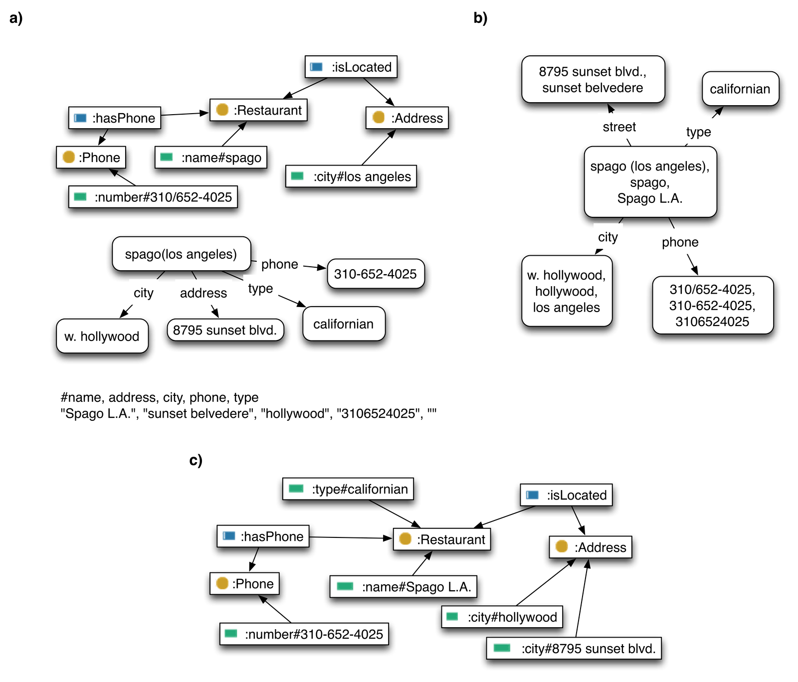
Figure 5.2: Entity resolution and redundancy elimination on three knowledge chunks (see Section 3.2). a) Input data in a form of ontology (see Figure 3.2), network and attribute values. b) Cluster network obtained with entity resolution (i.e. matching). c) Final ontology obtained after redundancy elimination and appropriate postprocessing.
Let \(c\in C\) be a cluster representing some entity on abstract level (resolved in the previous step), let \(k_1,k_2\dots k_n\in c\) be its knowledge chunks and let \(k^c\) be the merged knowledge chunk, we wish to obtain. Furthermore, for some attribute \(a \in A_ \cdot\), let \(X^a\) be a random variable measuring the true value of \(a\) and let \(X_i^a\) be the random variables for \(a\) in each knowledge chunk it occurs (i.e. \(k_i.a\)). Value of attribute \(a\) for the merged knowledge chunk \(k^c\) is then defined as
\[\begin{equation} \operatorname*{arg\,max}_v P(X^a=v|\bigwedge_i X_i^a=k_i.a). \tag{5.10} \end{equation}\]Each attribute is thus assigned the most probable value, given the evidence observed (i.e. values \(k_i.a\)). By assuming pair-wise independence among \(X_i^a\) (conditional on \(X^a\)) and uniform distribution of \(X^a\) equation (5.10) simplifies to
\[\begin{equation} \operatorname*{arg\,max}_v\prod_i P(X_i^a=k_i.a|X^a=v). \tag{5.11} %\operatorname*{arg\,max}_v\frac{P(A=v)\prod_i P(A_i=k_i.a|A=v)}{\prod_i P(A_i=k_i.a)} %P(A|A_1,A_2\dots A_n) & = & \frac{P(A)\prod_{i=1}^n P(A_i|A)}{\prod_{i=1}^n P(A_i)} \end{equation}\]Finally, conditional probabilities in equation (5.11) are approximated with trustworthiness of values,
\[\begin{equation} \tag{5.12} P(X_i^a|X^a) \approx \begin{cases} T(k_i.a) & \text{for } k_i.a=v,\\ 1-T(k_i.a) & \text{for } k_i.a\neq v \end{cases} \end{equation}\]hence
\[\begin{equation} k^c.a = \operatorname*{arg\,max}_v\prod_{k_i.a=v} T(k_i.a)\prod_{k_i.a\neq v} 1-T(k_i.a). \tag{5.13} \end{equation}\]Only knowledge chunks (see section 3.2) containing attribute \(a\) are considered.
In the following we present the proposed redundancy elimination algorithm 5.2.
The algorithm uses knowledge chunk representation of semantic level. First, it initializes merged knowledge chunks \(k^c\in K^C\). Then, for each attribute \(k^c.a\), it finds the most probable value among all given knowledge chunks (line \(3\)). When the algorithm unfolds, knowledge chunks \(K^C\) represent a merged dataset, with resolved entities and eliminated redundancy. Each knowledge chunk \(k^c\) corresponds to unique entity on abstract level, and each attribute holds the most trustworthy value.
At the end, only the data that was actually provided by some data source, should be preserved. Thus all inferred data (through \(\mathcal{I}_N\) or \(\mathcal{I}_O\); see section 3.3) is discarded, as it is merely an artificial representation needed for (common) entity resolution and redundancy elimination. Still, all provided data and semantical information is preserved and properly merged with the rest. Hence, although redundancy elimination is done on semantic level, resulting dataset is given on both data and semantic level (that complement each other).
Last, we discuss the assumptions of independence among \(X_i^a\) and uniform distribution of \(X^a\). Clearly, both assumptions are violated, still the former must be made in order for the computation of most probable value to be feasible. However, the latter can be eliminated when distribution of \(X^a\) can be approximated from some large-enough dataset.
5.4 General framework
Proposed entity resolution and redundancy elimination algorithms (see sections 5.2 and 5.3) are integrated into a general framework for matching and merging (see Figure 5.3). Framework represents a complete solution, allowing a joint control over various dimensions of matching and merging execution. Each component of the framework is briefly presented in the following, and further discussed in section 7.
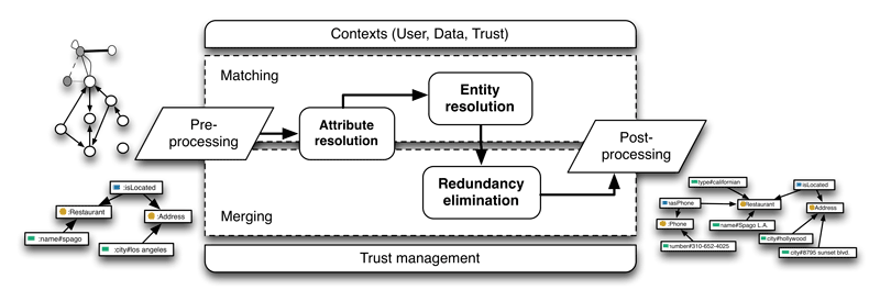
Figure 5.3: General framework for matching and merging data from heterogeneous sources.
Initially, data from various sources is preprocessed appropriately. Every network or ontology is transformed into a knowledge chunk representation and, when needed, also inferred on an absent architecture level (see section 3.3). After preprocessing is done, all data is represented in the same, easily manageable, form, allowing for common, semantically elevated, subsequent analyses.
Prior to entity resolution, attribute resolution is done (see section 5.2). The process resolves and matches attributes in the heterogeneous datasets, using the same algorithm as for entity resolution. As all data is represented in the form of knowledge chunks, this actually unifies all the underlying networks and ontologies.
Next, proposed entity resolution and redundancy elimination algorithms are employed (see sections 5.2 and 5.3). The process thus first resolves entities in the data, and then uses this information to eliminate the redundancy and to merge the datasets at hand. Algorithms explore not only the related data, but also the semantics behind it, to further improve the performance.
Last, postprocessing is done, in order to discard all artificially inferred data and to translate knowledge chunks back to the original network or ontology representation (see section 3). Throughout the entire execution, components are jointly controlled through (defined) user, data and trust contexts (see section 5.1). Furthermore, contexts also manage the results of the algorithms, to account for specific needs of each scenario.
Every component of the framework is further enhanced, to allow for proper trust management, and thus also for efficient security assurance. In particular, all the similarity measures for entity resolution are trust-aware, moreover, trust is even used as a primary evidence in the redundancy elimination algorithm. The introduction of trust-aware and security-aware algorithms represents the main novelty of the proposition.
6 Experiments
In the following subsections we demonstrate the framework’s (see Figure 5.3) most important parts on several real-world datasets, designed for entity resolution tasks and discuss the results. The part of attribute resolution and redundancy elimination evaluation is shown like a case study because to our knowledge, no tagged data combining all results we need, exists.
The demonstration is done with respect to semantic elevation, semantic similarity and trust management contexts (see section 5.1). We do not fit methods for the datasets to achieve superior performance, but rather focus on the increase of accuracy when using each of the contexts. In the following we present the datasets, explain used metrics, show the results and discuss them. The used datasets and full source code is publicly available5.
6.1 Datasets
We consider five testbeds of four different domains to simulate real-life matching tasks. Each data source introduces many data quality problems, in particular duplicate references, heterogeneous representations, misspellings or extraction errors.
The CiteSeer dataset used is a cleaned version6 from Getoor L. et. al. (Bhattacharya and Getoor 2007), others were presented and evaluated against entity resolution algorithms by Köpcke, Thor, and Rahm (2010)7.
- CiteSeer dataset contains \(1,504\) machine learning documents with \(2,892\) author references to \(1,165\) author entities. The only attribute information available is name for authors and title for documents.
- DBLP-ACM dataset consists of two well-structured bibliographic data sources from DBLP and ACM with 2616 and 2294 references to 2224 document entities. Each reference contains values for title, authors, venue and publication year of respective scientific paper.
- Restaurants dataset contains \(864\) references to \(754\) restaurant entities. Most of the references contain values for name, address, city, phone number and type of certain restaurant.
- AbtBuy is an e-commerce dataset with extracted data from Abt.com and Buy.com. They contain \(1,081\) and \(1,092\) references to 1097 different products. Each product reference is mostly represented by product name, manufacturer and often missing description and price values.
- Affiliations dataset consists of \(2,260\) references to \(331\) organizations. The only attribute value per record is an organization name, which can be written in many possible ways (i.e. full, part name or abbreviation).
6.2 Attribute resolution
As a part of semantic elevation, the input datasets must be aligned by attribute-value pairs to achieve a mutual representation. As mentioned in section 5.2, an entity resolution algorithm could be used to merge appropriate attributes. To better solve the problem in general, we propose the following similarity functions:
- ExactMatch: The simplest version. Attribute names must match exactly.
- SimilarityMatch: Every two attributes with score above the selected threshold, are matched (We use Jaro-Winkler (Winkler 1990) metric with threshold of \(0.95\)). This is typical pairwise entity resolution approach.
- SimilarityMatch+: In addition to previous function, it considers synonyms when comparing two attribute names (synsets from semantic lexicon Wordnet (Miller 1995) are used). Real-life datasets along with attribute names are created by people and that is why attributes over different datasets are supposed to be synonyms.
- DomainMatch: Same attribute values contain similar data format. Leveraging this information we extract selected features and match the most similar attributes across datasets. (A simple example is calculating the average number of words per attribute values.)
- OntologyMatch: Using ontologies, additional semantic information is included. If all input datasets are semantically described using ontologies, related data types
sameAsorseeAlso, possible hierarchy of subclasses, included rules and axioms can be additionally used for matching. When none of this apply, previous procedures must be employed.
As our datasets mostly consist of \(2\) different already aligned sources, we have chosen some additional attribute names for DBLP-ACM dataset manually. Altered values are shown in Table 6.1. Due to space limitations, we just presentively discuss the results. First line are the original attribute names and next three lines are changed to show success of proposed matchers. Pair \((1,2)\) is successfully solved by SimilarityMatch. The difference between values is limited to misspellings and small writing errors. Pair \((1,3)\) is a bit more difficult. Values authors and writers or year and yr cannot be matched by similarity. As they are synonyms, SimilarityMatch+ can match them. Pair \((1,4)\) values are completely different and it is completely useless to check name pairs. The DomainMatch technique correctly matches the attributes by considering attribute values format.
| id | #1 | #2 | #3 | #4 |
|---|---|---|---|---|
| 1 | title | venue | year | authors |
| 2 | titl | venue | year | author |
| 3 | title | venue | yr | writers |
| 4 | attr1 | attr2 | attr3 | attr4 |
6.3 Entity resolution
In this section we first discuss the selected entity resolution algorithm and then show the increase in correctly matched values using semantic similarity. We implemented the algorithm, proposed in (Bhattacharya and Getoor 2007), which is well described in section 5.2 and presented as algorithm 5.2.
In addition to the standard blocking techniques of partially string matching we added similarity, n-gram blocking and also enabled the option of fuzzy blocking. Standard approach is used on AbtBuy, CiteSeer and DBLP-ACM datasets. Similarity blocking adds an instance to a block if the similarity score with the representative reference of the block is above the defined threshold. This type of blocking was used with the Restaurants dataset using \(0.3\) threshold for name and \(0.7\) for phone attribute. At Affiliations dataset we use n-gram blocking with at least \(4\) \(6\)-gram matches.
We use secondstring (Cohen, Ravikumar, and Fienberg 2003) library for all basic similarity measures implementations. At bootstrapping and clustering we use JaroWinkler with TFIDF and manual weights as an attribute metric. Promising general results were achieved also using n-gram and Level2JaroWinkler metric. As a related similarity we use k-Neighbours at bootstrapping and modified JaccardCoefficient at clustering. The modification just aligns the match result \(x\) using function \(f(x) = -(-x+1)^{10}+1\), because similarity pairs instead of typical sets are checked.
The most important parameters that need to be selected are similarity alpha \(\alpha\) and merge threshold \(\theta_S\). Both values were selected subjectively and not dataset - specific. We set similarity alpha to \(\alpha = 0.85\), which results in weighting attribute metric to \(\delta_A = \alpha\) and related data metric to \(\delta_R = 1-\alpha\). Matching accuracy using different similarity alphas is shown on Figure 6.1. As it can be seen from the figure, some datasets contain a lot of disambiguate values, which results in very low F-score at \(\alpha\) set to \(1\).
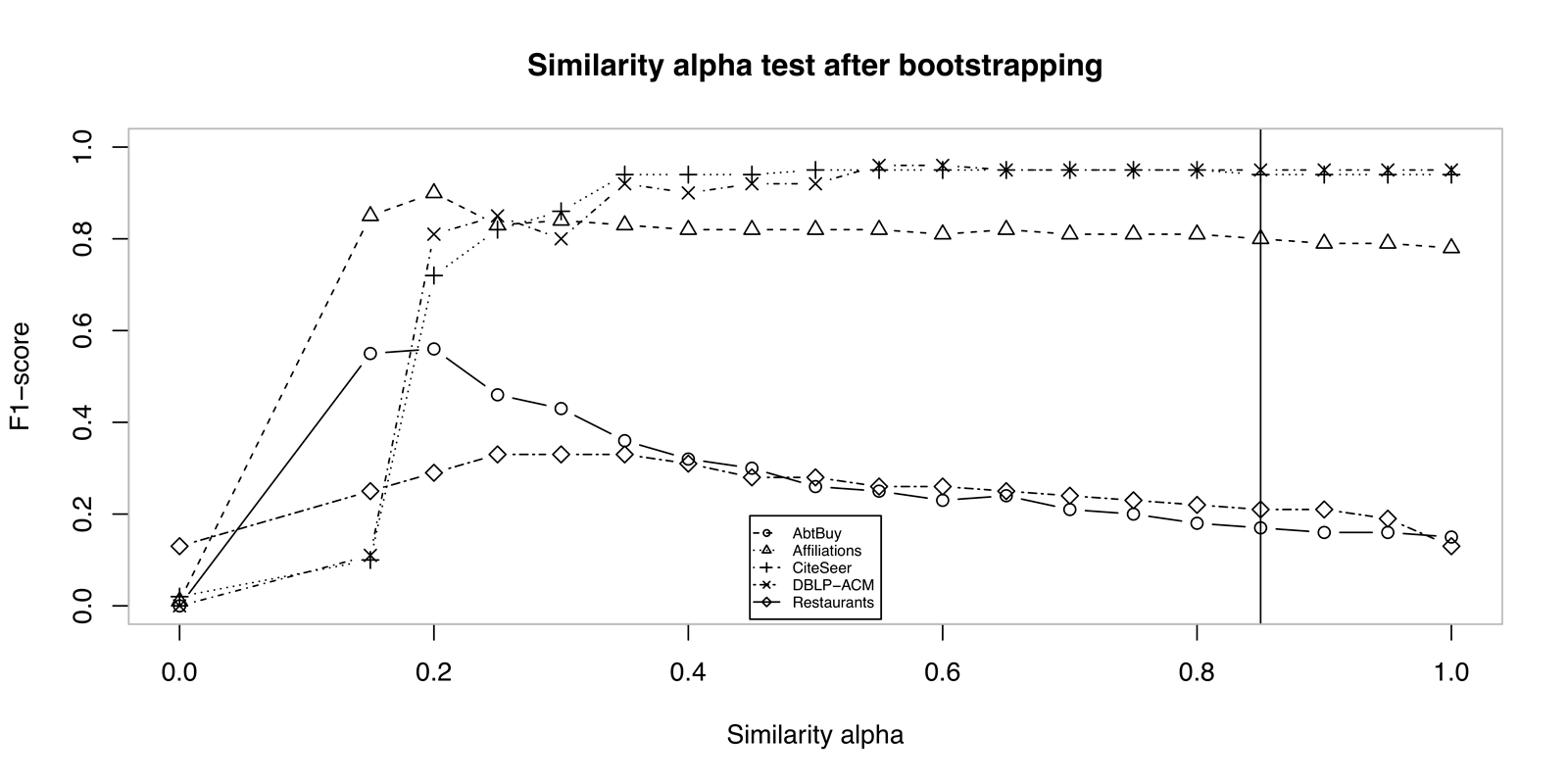
Figure 6.1: Comparison of entity resolution results after bootstrapping according to similarity alpha.
Merge threshold in our solution is set to \(0.95\). Testing the threshold at different values after bootstrapping is presented on Figure 6.2 and after clustering on Figure 6.3. It is possible to see the effect of iterative matching and related data metric from the Figure 6.3, which improves the final results. During testing these parameters, no semantic measure was used yet.
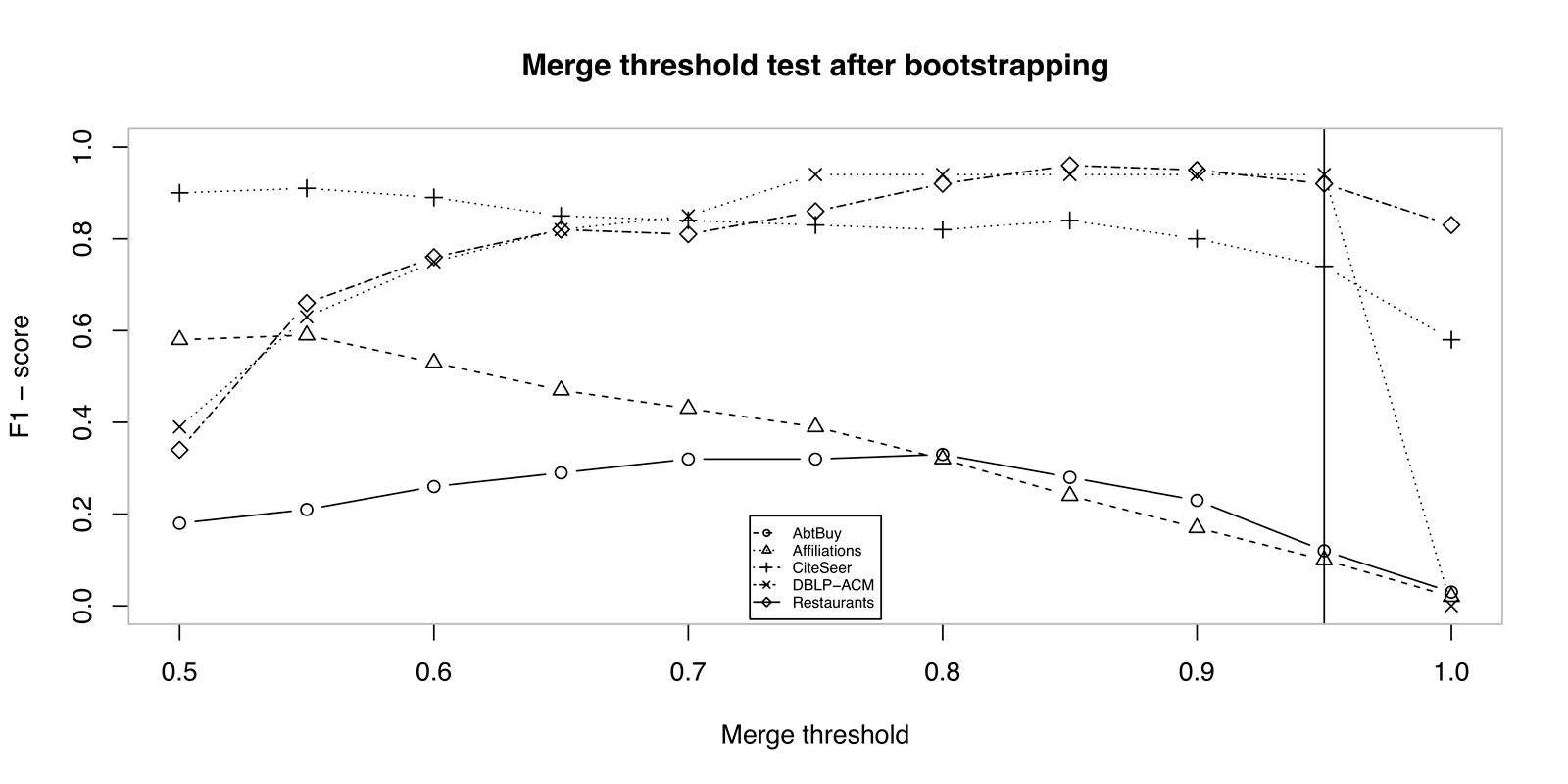
Figure 6.2: Comparison of entity resolution results after bootstrapping according to \(\theta_S\) merge threshold.
Figure 6.3: Comparison of entity resolution results after clustering according to \(\theta_S\) merge threshold.
Due to optimization, our implementation updates or possibly inserts only neighbour pairs of matched clusters into priority queue during clustering. The accuracy when checking only neighbours remains unchanged. Therefore the cluster \(c_k \in nbr(c_i \cup c_j)\) at the \(19^{th}\) line of algorithm 5.1).
On Figures 6.4 and 6.5 we present the increase of success in matching using semantic similarity (see Equation (5.8)). We set semantic similarity weight \(\delta_s\) to \(4\) based on some preliminary experiments. Getoor et. al. (Bhattacharya and Getoor 2007) adjusted Adar (Adamic and Adar 2001) similarity metric to better support values (e.g. author names) disambiguation. It learns an ambiguity function after checking the whole set of values in the dataset, similar to TF-IDF approach. This metric better models names, but does not use semantics, like identifying first or last name, product codes or specific parts of given value. Semantic similarity should model the human reasoning whether to match two values or not. For better understanding the meaning of semantic similarity, we present few examples, used in the experiment:
- Name metric: This is our the most general similarity metric. It models typical value matching by splitting it into tokens, identifying the value with less information and comparing it to other value’s tokens by startWith or similarity metric. It also checks and matches abbreviations. For example, every pair of names “William Cohen”, “W. Cohen”, “W.W. Cohen” or “Cohen” must have maximum semantic similarity. Similar applies to “Arizona State Univ., Tempe, AZ”, “Arizona State University” and “Arizona State University, Arizona” where using string similarity metric yields low values. Name metric is used for organization name matching on Affilation dataset, author name matching on CiteSeer and phone and restaurant name matching on Restaurants dataset.
- Number metric: Number metric identifies numeric values and matches them according to difference in values. It is used on DBLP-ACM dataset at publication year matching.
- Product metric: Product metric is designed to match products, which sometimes contain serial numbers or codes. These codes are commonly represented as a sequence of numbers and/or letters. In addition to code matching, it integrates Name metric with minimum \(k\) token match score. An example of matching two products is “Toshiba 40’ Black Flat Panel LCD HDTV - 40RV525U” and “Toshiba 40RV525U - 40’ Widescreen 1080p LCD HDTV w/ Cinespeed - Piano Black” where it is very hard to identity pair without code detection. Product metric is used on AbtBuy dataset for product name matching.
- Restaurant metric: This metric is specific to Restaurants dataset. It supposes attributes name and phone or location are scored above the threshold to match.
- Title metric: Titles are sometimes shrinked, have some words replaced with synonyms or refer to papers, written in more parts. This metric improves matching titles on DBLP-ACM dataset.
Figure 6.4: Comparison of entity resolution results after bootstrapping without and with using semantic similarity.
Figure 6.5: Comparison of entity resolution results after clustering without and with using semantic similarity.
The results on Figures 6.4 and 6.5 show the increase of matching accuracy by employing semantic similarity measure. The results on AbtBuy dataset are increased by \(11\%\) after clustering. Recall is significantly higher, but precision falls down. It is interesting that using semantics, same result is achieved immediately after bootstrapping, which shows good work at blocking. On Affiliations, the precision lowers, but employing semantics, more organizations with different name representations are resolved. CiteSeer gains more than \(10\%\) in recall and F-score and also keeps all measures above \(90\%\). At DBLP-ACM dataset, the differences are not very significant, but use of semantics still shows minor improvements. After bootstrapping at CiteSeer dataset it is interesting semantic similarity helps achieving \(100\%\) precision and a little improves the final result.
Experimenting using only semantic similarity metric gave worse results than including also attribute one. This is because our semantic similarities focus on semantics and not on misspelled or disambiguated data on lexical level. Restaurant dataset for example contains examples unsolvable even for a man without background knowledge. In the case of AbtBuy dataset even more knowledge would not work as name and product description is too general to match on some examples. Number match metric could be applied also on it, but one of the datasets barely contains a product’s price.
6.4 Redundancy elimination
The last step before postprocessing is merging knowledge chunks matched in clusters at entity resolution.
Merging is done entirely using trust management. In section 4 we define trust on levels of data source, knowledge chunk and value. As trust cannot be easily initialized, we select the appropriate cluster representative using trust of value only. Therefore we implemented the calculation of trust value for algorithm 5.2 in the following ways:
- Random: Random value is selected as the representative.
- Naive: Value that occurs the most time is selected as the representative.
- Naive+: The representative is selected as the maximum similar value to all others. Let \(c\) be a cluster of matched values, \(k\) value in cluster and Sim appropriate similarity function. Then the value is selected according to Equation (6.1). As similarity function we use Jaro-Winkler.
- Trust: Intuitively, a value is trustworthy if it yields many search results on the internet. This is not exactly true as for example the number of search results for “A. N.” is much higher comparing to “Andrew Ng”. By investigating some person name - based test searches, we expect the number of search hits decreases a lot if the word is misspelled. We denote \(N_{hits}(v)\) as the number of hits for value \(v\). Let \(N_{nhits}(v)\) be number of hits for a value of \(v\) with some noise added. We set \(m\) to \(5\) and change \(4\) letters or numbers randomly. The trust is calculated as in Equation (6.2) and as the result, the maximum trust value is selected.
During experiments, random clusters, having more than \(10\) values of specific attribute were selected for redundancy elimination. Using clusters with multiple values, the results are more representative because it is harder to select the right value. In each cluster, we add noise to a portion of values. So, one of the non-noise values is expected to be returned as a result of redundancy elimination because they certainly better represent the entity and this is taken as a measure of classification accuracy.
Author name attribute redundancy elimination results are presented on Figure 6.6 and in Table 6.2. The trust measure achieves better results comparing to others. It is expected for accuracy to be inversely proportional to level of noise, but the classification accuracy of the trust is above \(70\%\) even with \(90\%\) of noise in data. As we see, the trust measure outperforms other approaches throughout the test. The naive measure gives almost constant accuracy at all times. Naive+ approach performs vey bad by increasing the number of noise values. The reason it works better than naive at low noise levels is that there are many similar or equal values in cluster, but at higher levels, the majority of values are quite different. It’s results are similar to the random measure. Random approach results are expected, maybe even too good with clusters of a lot of noise. When having no knowledge of cluster values, performance of redundancy elimination would equal to random approach.
Figure 6.6: Redundancy elimination on CiteSeer dataset for \(34\) random clusters (as a result of ER), containing author names.
| Noise | Mean | Std. d. | Mean | Std. d. | Mean | Std. d. | Mean | Std. d. |
|---|---|---|---|---|---|---|---|---|
| 90% | 0.37 | 0.078 | 0.41 | 0.083 | 0.17 | 0.063 | 0.74 | 0.084 |
| 80% | 0.47 | 0.074 | 0.43 | 0.067 | 0.31 | 0.074 | 0.78 | 0.067 |
| 70% | 0.47 | 0.069 | 0.43 | 0.075 | 0.39 | 0.070 | 0.82 | 0.046 |
| 60% | 0.54 | 0.064 | 0.42 | 0.082 | 0.45 | 0.076 | 0.82 | 0.036 |
| 50% | 0.58 | 0.062 | 0.40 | 0.084 | 0.56 | 0.081 | 0.87 | 0.033 |
| 40% | 0.62 | 0.067 | 0.42 | 0.071 | 0.67 | 0.071 | 0.88 | 0.038 |
| 30% | 0.70 | 0.062 | 0.41 | 0.083 | 0.71 | 0.075 | 0.94 | 0.032 |
| 20% | 0.82 | 0.038 | 0.41 | 0.078 | 0.81 | 0.061 | 0.94 | 0.038 |
| 10% | 0.88 | 0.038 | 0.42 | 0.063 | 0.89 | 0.050 | 0.95 | 0.044 |
The experiment shows it may be easy to get useful redundancy eliminator for specific types of values, but the solution remains to initialize trust levels across the domain and update them continuously during system’s lifetime.
6.5 Experiments summary
We presented some experiments on the attribute, entity resolution and redundancy elimination components of the proposed general framework for matching and merging (see Figure 5.3).
As first, attribute resolution matches the datasets to the same semantic representation (see section 6.2). When datasets are not appropriately matched, missing attribute pairs cannot even be compared or wrong values are considered. Therefore, further matching strongly depends on attribute resolution result.
Second, we showed entity resolution improves if additional semantic similarity measure is used (see section 6.3). Semantic similarity is attribute type-specific and cannot be defined in general. Thus, a number of metrics could be predefined and then selected for each attribute type.
Third, input to redundancy elimination are clusters as a result from entity resolution (see section 6.4). For author names, we showed the search engine results as a value of trust, can help us determine the most appropriate value. Also, this component’s results strongly depend on matched clusters results as only one value within specific cluster can be selected.
To summarize, best evaluation measuring interdependence between components could be achieved only when having a dataset annotated with all needed contexts we defined. The proposed framework can be employed for general tasks, but would be outperformed by domain-specific applications.
7 Discussion
Proposed framework for matching and merging represents a general and complete solution, applicable in all diverse areas of use. Introduction of contexts allows a joint control over various dimensions of matching and merging variability, providing for specific needs of each scenario. Furthermore, data architecture combines simple (network) data with semantically enriched data, which makes the proposition applicable for any data source. Framework can thus be used as a general solution for merging data from heterogeneous sources, and also merely for matching.
The fundamental difference between matching, including only attribute and entity resolution, and merging, including also redundancy elimination, is, besides the obvious, in the fact that merged data is read-only. Since datasets, obtained after merging, do not necessarily resemble the original datasets, the data cannot be altered thus the changes would apply also in the original datasets. Alternative approach is to merely match the given datasets and to merge them only on demand. When altering matched data, user can change the original datasets (that are in this phase still represented independently) or change the merged dataset (that was previously demanded for), in which case he must also provide an appropriate strategy, how the changes should be applied in the original datasets.
Proposed algorithms employ network data, semantically enriched with ontologies. With the advent of Semantic Web, ontologies are gaining importance mainly due to availability of formal ontology languages. These standardization efforts promote several notable uses of ontologies like assisting in communication between people, achieving interoperability (communication) among heterogeneous software systems and improving the design and quality of software systems. One of the most prominent applications is in the domain of semantic interoperability. While pure semantics concerns the study of meanings, semantic elevation means to achieve semantic interoperability and can be considered as a subset of information integration (including data access, aggregation, correlation and transformation). Semantic elevation of proposed matching and merging framework represents one major step towards this end.
Use of trust-aware techniques and algorithms introduces several key properties. Firstly, an adequate trust management provides means to deal with uncertain or questionable data sources, by modeling trustworthiness of each provided value appropriately. Secondly, algorithms jointly optimize not only entity resolution or redundancy elimination of provided datasets, but also the trustworthiness of the resulting datasets. The latter can substantially increase the accuracy. Thirdly, trustworthiness of data can be used also for security reasons, by seeing trustworthy values as more secure. Optimizing the trustworthiness of matching and merging thus also results in an efficient security assurance.
Although, contexts are merely a way to guide the execution of some algorithm, their definition is relatively different from that of any simple parameter. The execution is controlled with mere definition of the contexts, when in the case of parameters, it is controlled by assigning different values. For instance, when default behavior is desired, the parameters still need to be assigned, when in the case of contexts, the algorithm is used as it is. For any general solution, working with heterogeneous clients, such behavior can significantly reduce the complexity.
As different contexts are used jointly throughout matching and merging execution, they allow a collective control over various dimensions of variability. Furthermore, each execution is controlled and also characterized with the context it defines, which can be used to compare and analyze different executions or matching and merging algorithms.
Last, we briefly discuss a possible disadvantage of the proposed framework. As the framework represents a general solution, applicable in all diverse domains, the performance of some domain-specific approach or algorithm can still be superior. However, such approaches commonly cannot be generalized and are thus inappropriate for practical (general) use.
8 Conclusion
This paper advances previously published paper (Šubelj et al. 2011) which contains only theoretical view of the proposed framework for data matching and merging. In this work we again overview the whole framework with minor changes, but most importantly we introduce different metrics implementation details and full framework demonstration.
The proposed framework follows a three level architecture using network-based data representation from data to semantic and lastly to abstract level. Data on each level is always a superset of lower ones due to inclusion of various context types, trust values or additional metadata. We also identify three main context types – user, data and trust context type – which are a formal representation of all possible operations. One of the novelties is also trust management that is available across all steps during the execution.
To support our framework proposal, we conduct experiments of three main components – attribute resolution, entity resolution and redundancy elimination – using trust and semantics. Like we theoretically anticipated, results on five datasets show that semantic elevation and proper trust management significantly improve overall results.
In further work we will additionally incorporate network analysis techniques such as community detection (Šubelj and Bajec 2011a) or recent research on self-similar networks (Blagus, Šubelj, and Bajec 2012), which finds network hierarchies with a number of common properties that may also improve the results of proposed approach. Furthermore, ontology-based information extraction techniques will be employed into entity resolution algorithm to gain more knowledge about non-atomic values.
Acknowledgement
We would also like to thank co-authors of the previous paper (Šubelj et al. 2011) – David Jelenc, Eva Zupančič, Denis Trček and Marjan Krisper – who have helped us with theoretical knowledge at framework design stage.
The work has been supported by the Slovene Research Agency ARRS within the research program P2-0359 and part financed by the European Union, European Social Fund.
References
Adamic, L., and E. Adar. 2001. “Friends and Neighbors on the Web.” Social Networks 25: 211–30.
Ananthakrishna, Rohit, Surajit Chaudhuri, and Venkatesh Ganti. 2002. “Eliminating Fuzzy Duplicates in Data Warehouses.” In Proceedings of the International Conference on Very Large Data Bases, 586–97.
Bengtson, Eric, and Dan Roth. 2008. “Understanding the Value of Features for Coreference Resolution.” In Proceedings of the Conference on Empirical Methods in Natural Language Processing, 294–303. Association for Computational Linguistics.
Bhattacharya, Indrajit, and Lise Getoor. 2004. “Iterative Record Linkage for Cleaning and Integration.” In Proceedings of the ACM SIGKDD Workshop on Research Issues in Data Mining and Knowledge Discovery, 11–18.
———. 2007. “Collective Entity Resolution in Relational Data.” ACM Transactions on Knowledge Discovery from Data 1 (1): 5.
Blagus, Neli, Lovro Šubelj, and Marko Bajec. 2012. “Self-Similar Scaling of Density in Complex Real-World Networks.” Physica A - Statistical Mechanics and Its Applications 391 (8): 2794–2802. doi:10.1016/j.physa.2011.12.055.
Blaze Software. 1999. “Blaze Advisor.” Technical White Paper, version 2.5. http://condor.depaul.edu/jtullis/documents/Blaze_Advisor_Tech.pdf.
Castano, Silvana, Alfio Ferrara, and Stefano Montanelli. 2006. “Matching Ontologies in Open Networked Systems: Techniques and Applications.” Journal on Data Semantics, 25–63.
———. 2009. “The iCoord Knowledge Model for P2P Semantic Coordination.” In Proceedings of the Conference on Italian Chapter of AIS.
———. 2010. “Dealing with Matching Variability of Semantic Web Data Using Contexts.” In Proceedings of the International Conference on Advanced Information Systems Engineering.
Chakrabarti, Soumen, Byron Dom, Prabhakar Raghavan, Sridhar Rajagopalan, D. Gibson, and J. Keinberg. 1998. “Automatic Resource Compilation by Analyzing Hyperlink Structure and Associated Text.” Proceedings of the International World Wide Web Conference, 65–74.
Cohen, William W. 2000. “Data Integration Using Similarity Joins and a Word-Based Information Representation Language.” ACM Transactions on Information Systems 18 (3): 288–321.
Cohen, William W., Pradeep Ravikumar, and Stephen E. Fienberg. 2003. “A Comparison of String Distance Metrics for Name-Matching Tasks.” In Proceedings of the IJCAI Workshop on Information Integration on the Web, 73–78.
Domingos, P., and M. Richardson. 2001. “Mining the Network Value of Customers.” In Proceedings of the International Conference on Knowledge Discovery and Data Mining, 57–66.
Dong, Xin, Alon Halevy, and Jayant Madhavan. 2005. “Reference Reconciliation in Complex Information Spaces.” In Proceedings of the ACM SIGMOD International Conference on Management of Data, 85–96.
Euzenat, JÈrÙme, and Pavel Shvaiko. 2007. Ontology Matching. Springer-Verlag.
Gruber, T. R. 1993. “A Translation Approach to Portable Ontology Specifications.” Knowledge Acquisition 5 (2): 199–220.
Hernandez, Mauricio, and Salvatore Stolfo. 1995. “The Merge/Purge Problem for Large Databases.” Proceedings of the ACM SIGMOD International Conference on Management of Data, 127–38.
Horrocks, Ian, and Ulrike Sattler. 2001. “Ontology Reasoning in the SHOQ (D) Description Logic.” In IJCAI, 1:199–204.
Jaro, M. A. 1989. “Advances in Record Linking Methodolg as Applied to the 1985 Census of Tampa Florida.” Journal of the American Statistical Society 84 (406): 414–20.
Kalashnikov, D., and S. Mehrotra. 2006. “Domain-Independent Data Cleaning via Anlysis of Entity-Relationship Graph.” ACM Transactions on Database Systems 31 (2): 716–67.
Kautz, Henry, Bart Selman, and Mehul Shah. 1997. “Referral Web: Combining Social Networks and Collaborative Filtering.” Communications of the ACM 40 (3): 63–65.
Köpcke, H., A. Thor, and E. Rahm. 2010. “Evaluation of Entity Resolution Approaches on Real-World Match Problems.” Proceedings of the VLDB Endowment 3 (1-2): 484–93.
Lapouchnian, Alexei, and John Mylopoulos. 2009. “Modeling Domain Variability in Requirements Engineering with Contexts.” In Proceedings of the International Conference on Conceptual Modeling, 115–30. Gramado, Brazil: Springer-Verlag.
Lavbič, Dejan, Olegas Vasilecas, and Rok Rupnik. 2010. “Ontology-Based Multi-Agent System to Support Business Users and Management.” Technological and Economic Development of Economy 16 (2): 327–47. doi:10.3846/tede.2010.21.
Lee, Heeyoung, Yves Peirsman, Angel Chang, Nathanael Chambers, Mihai Surdeanu, and Dan Jurafsky. 2011. “Stanford’s Multi-Pass Sieve Coreference Resolution System at the CoNLL-2011 Shared Task.” In Proceedings of the Fifteenth Conference on Computational Natural Language Learning: Shared Task, 28–34. Association for Computational Linguistics.
Lenzerini, Maurizio. 2002. “Data Integration: A Theoretical Perspective.” In Proceedings of the ACM SIGMOD Symposium on Principles of Database Systems, 233–46.
Levenshtein, Vladimir. 1966. “Binary Codes Capable of Correcting Deletions, Insertions, and Reversals.” Soviet Physics Doklady 10 (8): 707–10.
Miller, George A. 1995. “WordNet: A Lexical Database for English.” Communications of the ACM 38 (11): 39–41.
Monge, Alvaro, and Charles Elkan. 1996. “The Field Matching Problem: Algorithms and Applications.” Proceedings of the International Conference on Knowledge Discovery and Data Mining, 267–70.
Moreau, Erwan, FranÁois Yvon, and Olivier CappÈ. 2008. “Robust Similarity Measures for Named Entities Matching.” In Proceedings of the International Conference on Computational Linguistics, 593–600.
Nagy, Miklos, Maria Vargas-Vera, and Enrico Motta. 2008. “Managing Conflicting Beliefs with Fuzzy Trust on the Semantic Web.” In Proceedings of the Mexican International Conference on Advances in Artificial Intelligence, 827–37.
Newman, Mej. 2010. Networks: An Introduction. Oxford University Press, Oxford.
Ng, Vincent. 2008. “Unsupervised Models for Coreference Resolution.” In Proceedings of the Conference on Empirical Methods in Natural Language Processing, 640–49. Association for Computational Linguistics.
Rahm, Erhard, and Philip A. Bernstein. 2001. “A Survey of Approaches to Automatic Schema Matching.” Journal on Very Large Data Bases 10 (4): 334–50.
Resnick, Paul, Neophytos Iacovou, Mitesh Suchak, Peter Bergstrom, and John Riedl. 1994. “GroupLens: An Open Architecture for Collaborative Filtering of Netnews.” In Proceedings of ACM Conference on Computer Supported Cooperative Work, 175–86.
Richardson, Matthew, Rakesh Agrawal, and Pedro Domingos. 2003. “Trust Management for the Semantic Web.” In Proceedings of the International Semantic Web Conference, 351–68.
Štajner, Tadej, and Dunja Mladenić. 2009. “Entity Resolution in Texts Using Statistical Learning and Ontologies.” In Asian Semantic Web Conference, 91–104. Springer.
Šubelj, Lovro, and Marko Bajec. 2011a. “Community Structure of Complex Software Systems: Analysis and Applications.” Physcia A - Statistical Mechanics and Its Applications 390 (16): 2968–75. doi:10.1016/j.physa.2011.03.036.
———. 2011b. “Robust Network Community Detection Using Balanced Propagation.” European Physical Journal B 81 (3): 353–62. doi:10.1140/epjb/e2011-10979-2.
Šubelj, Lovro, David Jelenc, Eva Zupančič, Dejan Lavbič, Denis Trček, Marjan Krisper, and Marko Bajec. 2011. “Merging Data Sources Based on Semantics, Contexts and Trust.” IPSI BgD Transactions on Internet Research 7 (1): 18–30.
Thor, Andreas, and Erhard Rahm. 2007. “Moma - a Mapping-Based Object Matching System.” In Proceedings of the 3rd Biennial Conference on Innovative Data Systems Research.
Trček, Denis. 2009. “A Formal Apparatus for Modeling Trust in Computing Environments.” Mathematical and Computer Modelling 49 (1-2): 226–33.
Whang, S., D. Marmaros, and H. Garcia-Molina. 2010. “Pay-as-You-Go ER.”
Whang, Steven Euijong, and Hector Garcia-Molina. 2013. “Disinformation Techniques for Entity Resolution.” In Proceedings of the 22nd ACM International Conference on Information & Knowledge Management, 715–20. ACM.
Winkler, William E. 1990. “String Comparator Metrics and Enhanced Decision Rules in the Fellegi-Sunter Model of Record Linkage.” In Proceedings of the Section on Survey Research Methods, 354–59.
Resource Description Framework Schema↩
Web Ontology Language↩
Hypergraphs are graphs, where edges can connect multiple vertices.↩
Term Frequency-Inverse Document Frequency↩
http://www.cs.umd.edu/projects/linqs/projects/er/DATA/citeseer.dat↩
http://dbs.uni-leipzig.de/en/research/projects/object_matching/fever/benchmark_datasets_for_entity_resolution↩