What language do stocks speak?
Marko Poženel and Dejan Lavbič. 2018. What language do stocks speak?, 13th International Baltic Conference on Databases and Information Systems (Baltic DB&IS 2018), 1. 7. 2018 - 4. 7. 2018, Trakai, Lithuania.
Abstract
Stock prediction is a challenging and chaotic research area where many variables are included with their effects being complex to determine. Nevertheless, stock value prediction is still very appealing for researchers and investors since it might be profitable, yet the number of published research papers remains to be relatively small. The employment of advanced data analysis techniques has already been suggested by previous researches, such as the use of neural networks for stock price prediction, but practical implications of the the majority of approaches are limited as they are concerned mainly with a prediction accuracy and less with the success in real trading with consideration of trading fees. We propose a novel approach for stock trend prediction that combines Japanese candlesticks (OHLC trading data) and neural network based group of models Word2Vec. Word2Vec is usually utilized to produce word embeddings in natural language processing tasks, while we adopt it for acquiring semantic context of words in candlesticks’ sequence, where clustered candlesticks represent stock’s words. The approach is employed for the extraction of useful information from large sets of OHLC trading data to improve prediction accuracy. In evaluation of our approach we define a trading strategy and compare our approach with other popular prediction models – Buy & Hold, MA and MACD. The evaluation results on Russell Top 50 index are encouraging – the proposed Word2Vec approach outperformed all compared models on a test set with a statistical significance.
Keywords
Stock price prediction, Trading strategy, Word2Vec, NLP
1 Introduction
Forecasting trends and the future value of stocks has always been an interesting topic for both investors and research community. However, the number of successful researches and published papers is still very low. The reason is simple, usually nobody wants to publish an algorithm that solves one of the issues that might be most profitable. Nonetheless, there are many approaches to forecasting the future stock values, where the most influential are:
- technical analysis (Taylor and Allen 1992) and
- fundamental analysis (Abad, Thore, and Laffarga 2004).
Fundamental analysis of financial markets involves detailed analysis of the company’s business, various news about the enterprise and the prediction of future growth. It deals with linking current company’s financial data to future earnings and evaluation of how it will affect company’s value. A large number of factors have to be included in the evaluation (Abad, Thore, and Laffarga 2004). Several approaches that attempt to automate stock trading based on processing of unstructured text sources such as news articles, company reports or individual posts (Nassirtoussi et al. 2015; Huang et al. 2016; Shynkevich et al. 2016), are typically based on Natural Language Processing Algorithms (NPA).
The second approach to trading is based solely on the basis of historical price changes and technical analysis. Technical analysis provides data for trading decisions largely on the basis of visual inspection of past trend movements, without employing any part of fundamental analysis (Taylor and Allen 1992). Proponents of technical analysis claim that all necessary information for forecasting the stock price trends are already included in the stock price itself. They point out that events in the history are repeated and that stock prices can be forecasted based on current trends (Prado et al. 2013).
Very popular technical method to convey the growth and decline of the demand and supply in financial markets is the candlestick trading strategy (Lu and Shiu 2011; Nison 1991). It is one of the oldest technical analyses techniques with origins in \(18^{\text{th}}\) century where it was used by Munehisa Homma for trading with rice. He analysed rice prices back in time and acquired huge insights to the rice trading characteristics. Japanese candlestick charting technique is a primary tool to visualize the changes in a commodity price in a certain time span. Nowadays candlestick charting technique can be found in almost every software and on-line charting packages (Jasemi, Kimiagari, and Memariani 2011). Although the researchers are not in complete agreement about its efficiency, many researchers are investigating its potential use in various fields (Prado et al. 2013; Jasemi, Kimiagari, and Memariani 2011; Lu and Shiu 2012; Kamo and Dagli 2009; Lu 2014). To visualize Japanese candlestick at a certain time grain (e.g. day, hour), four key data components of a price are required: starting price, highest price, lowest price and closing price. This tuple is called OHLC (Open, High, Low, Close). Figure 1.1 shows an example of a Japanese white and black body candlestick with the notation used in this paper. When the candlestick body is filled, the closing price of the session was lower than the opening price. If the body is empty, the closing price was higher than the opening price. The thin lines above and below the rectangle body are called shadows and represent session’s price extremes. There are many types of Japanese candlesticks with their distinctive names. Figure 1.2 shows only some of the most commonly seen in candlestick charts. Each candlestick holds information on trading session and becomes even more important, when it is an integral part of certain sequence.
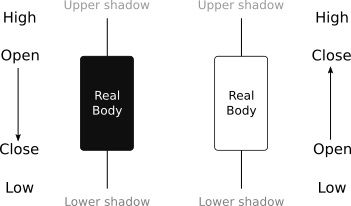
Figure 1.1: The presentation of Japanese candlestick

Figure 1.2: Some of the most popular Japanese candlesticks
The work presented in this paper is an attempt to create a simplified OHLC language (i.e. simplified language of Japanese candlesticks from OHLC data) that is later used as an input for Word2Vec algorithm (Mikolov, Sutskever, et al. 2013) that can learn the vector representations of words in the high-dimensional vector space. We believe that it is possible to learn rules and patterns using Word2Vec and use this knowledge to predict future trends in stock value. Despite many developed models and predictive techniques, measuring performance of the stock prediction models can present a challenge. For example, Jasemi et al. (Jasemi, Kimiagari, and Memariani 2011) used hit ratio to evaluate the performance of the models but neglected financial success of a model. Therefore, one of the research goals of this paper is also to utilize a simple method for testing the performance of forecasting models, the result of which is the financial success or yield of the tested model.
The remaining paper is organized as follows. Section 2 contains a literature overview. Section 3 is dedicated to a detailed overview of the proposed forecasting model. In Section 4 model evaluation and performance metrics are presented. Section 5 presents the conclusions and future work.
3 Proposed forecasting model
The proposed forecasting model that combines a set of machine learning methods in a novel and innovative way. The basic assumption behind the proposed approach is that Japanese candlesticks are not only powerful tool for visualizing OHLC data, but also contain predictive power (Jasemi, Kimiagari, and Memariani 2011; Lu and Shiu 2012; Kamo and Dagli 2009; Lu 2014).
Our approach exploits Japanese candlesticks where various sequences are used to forecast the value of a stock. Japanese candlesticks are interpreted as a foundation for stocks’ language, i.e. words. A language in general consists of words and patterns of words that can be further grouped into sentences that express some deeper meaning. The proposed model relies on the similarities with the natural language.
The forecasting process starts with a transformation of OHLC data into a simplified language of Japanese candlesticks, i.e. stocks’ language. The acquired language is then processed with the NLP algorithm Word2Vec (Mikolov, Sutskever, et al. 2013) where we train the model with given characteristics and the legality of the proposed stocks’ language. The trained model is then used to predict future trends in stock value. The approach is depicted in Figure 3.1, with detailed description provided in the following subsections.
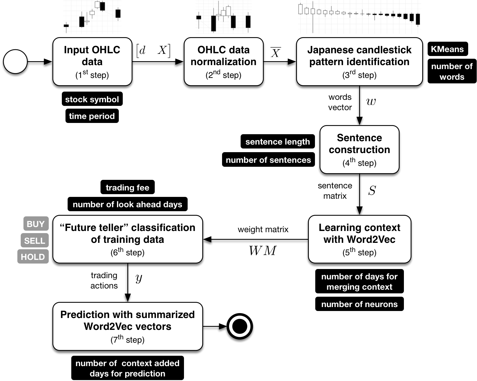
Figure 3.1: Steps of proposed forecasting model
3.1 Input OHLC data
For a given stock we observe the input data on a trading day basis for \(\boldsymbol{n_d}\) trading days as defined in the following matrix
\[\begin{equation} \begin{bmatrix} d_{(\text{$1$ $\times$ $n_d$})} & X_{(\text{$4$ $\times$ $n_d$})} \end{bmatrix} = \begin{bmatrix} \begin{array}{cc} d_1 \\ d_2 \\ \dots \\ d_{n_d} \end{array} \left| \begin{array}{*{4}c} O_1 & H_1 & L_1 & C_1 \\ O_2 & H_2 & L_2 & C_2 \\ \dots & \dots & \dots & \dots \\ O_{n_d} & H_{n_d} & L_{n_d} & C_{n_d} \end{array} \right. \end{bmatrix} \tag{3.1} \end{equation}\]where \(d_{(\text{$1$ $\times$ $n_d$})}\) is a vector of trading days and \(X_{(\text{$4$ $\times$ $n_d$})}\) is a matrix of OHLC trading data.
Japanese candlesticks are presented as OHLC tuples, where individual four attributes denote absolute value in time. Raw OHLC data in Equation (3.1) are convenient for graphical presentation (see Figure 3.2) but are not most suitable for further processing.
3.2 Data normalization
Since we are interested in the shape of Japanese candlesticks and not absolute value, the OHLC tuples were normalized by dividing OHLC data attributes (Open, High, Low, Close) with Open attribute as follows
\[\begin{equation} norm\big(\langle O,H,L,C \rangle\big) = \langle 1, \frac{H}{O}, \frac{L}{O}, \frac{C}{O}\rangle: X \to \overline{X} \tag{3.2} \end{equation}\]The employment of transformation from Equation (3.2) results in a new input trading data matrix
\[\begin{equation} \overline{X}_{(\text{$4$ $\times$ $n_d$})} = \begin{bmatrix} 1 & \frac{H_1}{O_1} & \frac{L_1}{O_1} & \frac{C_1}{O_1} \\\ 1 & \frac{H_2}{O_2} & \frac{L_2}{O_2} & \frac{C_2}{O_2} \\\ \dots & \dots & \dots & \dots \\\ 1 & \frac{H_{n_d}}{O_{n_d}} & \frac{L_{n_d}}{O_{n_d}} & \frac{C_{n_d}}{O_{n_d}} \end{bmatrix} \tag{3.3} \end{equation}\]where the shape of Japanese candlesticks is retained as depicted in Figure 3.3, while compared to Figure 3.2.
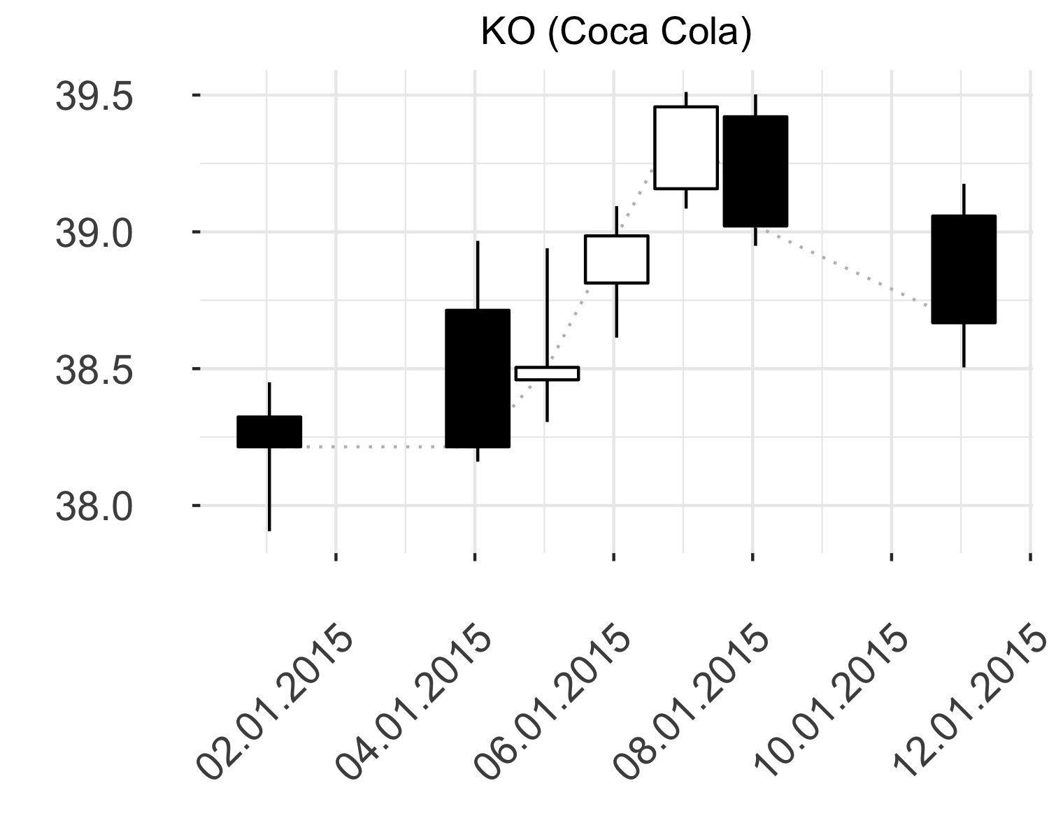
Figure 3.2: Raw OHLC data for stock KO in the begining of \(2015\)
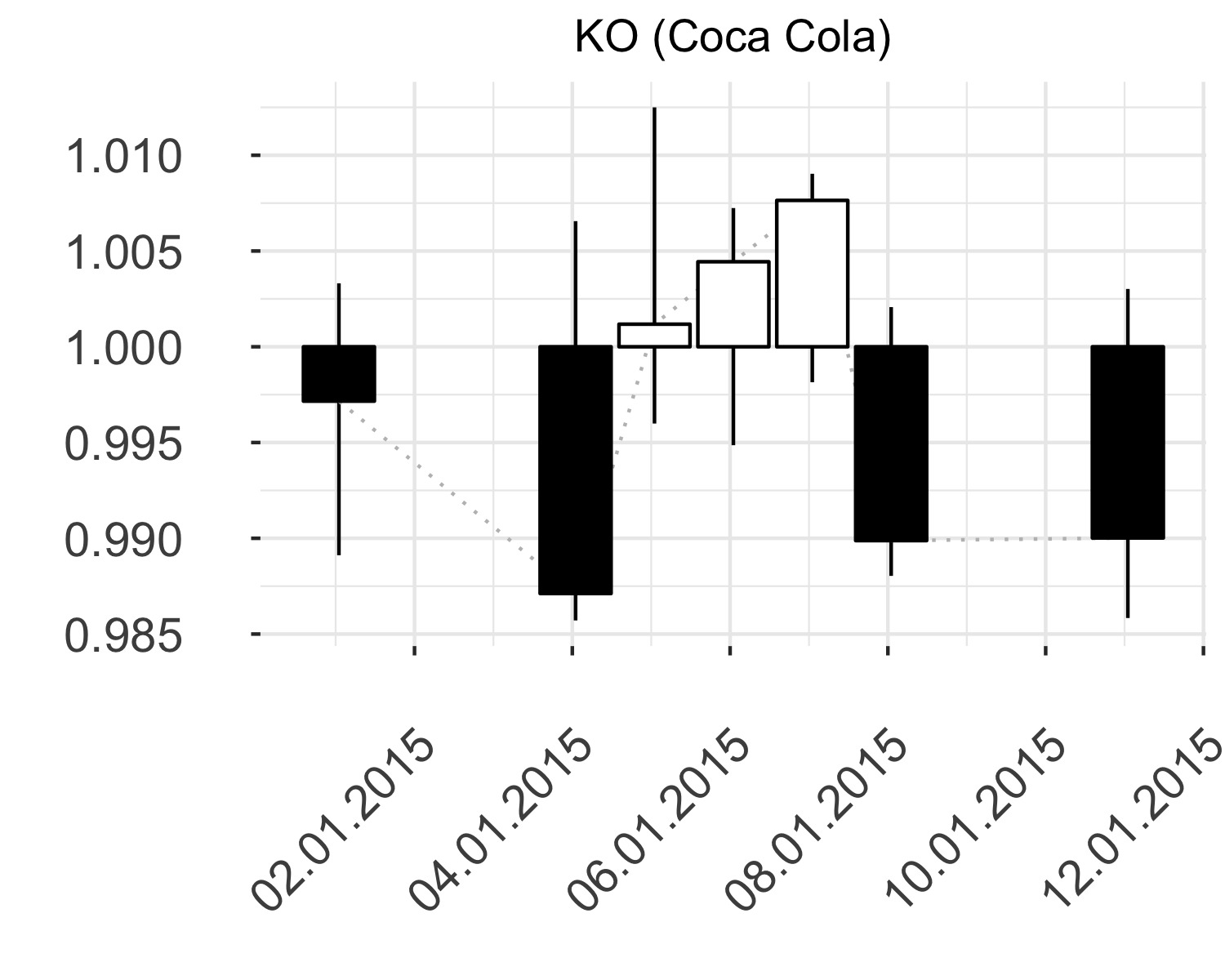
Figure 3.3: Normalized OHLC data for stock KO in the begining of \(2015\)
Figure 3.2 depicts raw OHLC data, where candlesticks are vertically positioned on the graph corresponding to their relative value. Figure 3.3 represents the same candlesticks after normalization process that emphasizes and retains the shape of individual candlestick.
3.3 Japanese candlestick pattern identification
Many forecasting models using Japanese candlesticks have a shortcoming of using predefined shapes of candlesticks (Martiny 2012). Therefore we have adopted the approach of automatically detecting candlestick clusters by employing unsupervised machine learning methods that performed well in previous research (Martiny 2012; Jasemi, Kimiagari, and Memariani 2011).
The rationale for using KMeans clustering was to limit the number of possible OHLC shapes (i.e. words of stocks’ language) while still being able to influence the unsupervised training process by setting the appropriate threshold for maximum number of different words.
In the process we define the maximum number of words in stocks’ language as \(\boldsymbol{n_w}\) and employ KMeans clustering algoritm to transform input data \(\overline{X}\) to vector \(w\) as follows
\[\begin{equation} KMeans\big(n_w\big): \overline{X} \to w \tag{3.4} \end{equation}\]where a word \(w_i\) is defined by an individual trading day \(\overline{X_i}\) and is a representation of a specific Japanese candlestick (the mean value of cluster \(i\)). The result of KMeans clustering is a vector
\[\begin{equation} w_{(\text{$1$ $\times$ $n_d$})} = \begin{bmatrix} w_1 & w_2 & \dots & w_{n_d} \end{bmatrix}^T \tag{3.5} \end{equation}\]where given word \(w_i\) is an element from a set of all possible Japanese candlesticks, where \(i = \big[1,n_w\big]\).
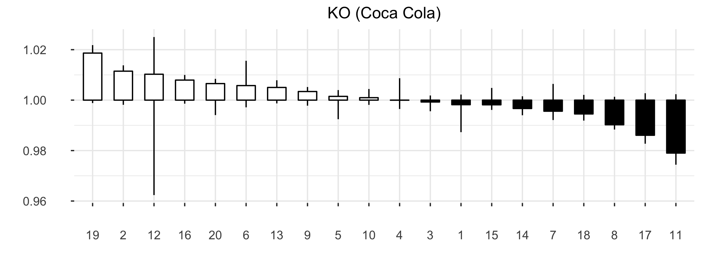
Figure 3.4: Example of \(20\) OHLC pattern clusters for stock KO
An example of a clustering process for a stock KO (Coca-Cola) is depicted in Fig. 3.4, where \(n_w = 20\) was used for maximum number of words. The value of parameter \(n_w\) is based on the Silhouette measure (Rousseeuw 1987), which shows how well an object lies in within a certain cluster (cohesion) compared to other clusters (separation). The Silhouette ranges from -1 to +1, where higher value of average Silhouettes means higher clustering validity. In defining stocks’ language our aim was also to retain the similarity of words that also exists in natural language by controlling \(n_w\) and the Silhouette measure.
3.4 Sentence construction
With numerous OHLC tuples the potential set of words for the stocks’ language is virtually infinite. In the previous section we have limited this to \(n_w\), which directly influences the performance of the proposed predictive model.
Looking at the analysis of past movements in the value of stock we can see that Japanese candlesticks’ sequences contain a certain predictive power (Nison 1991; Lu and Shiu 2012). Therefore, we considered past sequences of OHLC as a basis for the stock trend prediction by forming possible sentences in the future.
The proposed model does not contain any predefined rules for forecasting purposes. Rules used in further processing are created from sequences of patterns that are acquired from past movements in stock value.
We specify a sentence length \(\boldsymbol{l_s}\) that defines the number of consecutive words (i.e. trading days) grouped into sentences. The number of sentences \(\boldsymbol{n_s}\) is therefore dependent on the number of trading days \(n_d\) and the sentence length \(l_s\) and is defined as follows
\[\begin{equation} n_s = n_d - (l_s - 1) \tag{3.6} \end{equation}\]The result of the sentence construction process is a sentence matrix \(\boldsymbol{S}\) of rolling windows of trading data (more specifically words in stocks’ language from vector \(w\)) from a transformation \(w \to S\). Sentence matrix \(S\) with \(l_s\) columns (sentence length) and \(n_s\) rows (number of sentences) is further defined as
\[\begin{equation} S_{(\text{$l_s$ $\times$ $n_s$})} = \begin{bmatrix} w_1^{'} & w_2^{'} & \dots & w_{l_s}^{'} \\\ w_2^{'} & w_3^{'} & \dots & w_{l_s + 1}^{'} \\\ \dots & \dots & \dots & \dots \\\ w_{n_s}^{'} & w_{n_s + 1}^{'} & \dots & w_{n_d}^{'} \end{bmatrix} \tag{3.7} \end{equation}\]At first glance, such OHLC language seems very simple. However, considering the number of possible values for each word \(w_i\), a set of different possible sentences or patterns is enormous. We believe that the language thus defined has a high expressive power and is suitable for predictive purposes.
3.5 Learning context with Word2Vec
Based on the patterns in OHLC sentences, the model builds the language context that is then used to perform predictions in the following steps. The system employs historical data, recognizes existing patterns in sentences, learns the context of the words and also renews the context according to new acquired data by employing Word2Vec algorithm (Mikolov, Sutskever, et al. 2013) for training the context.
Word2Vec algorithm with skip-gram (Mikolov, Sutskever, et al. 2013; Mikolov, Chen, et al. 2013) uses a model to represent words with vectors from large amounts of unstructured text data. In the training process, Word2Vec acquires vectors for words that explicitly contain various linguistic rules and patterns by employment of neural network that contains only one hidden level, so it is relatively simple. Many of these patterns can be represented as linear translations. The Word2Vec algorithm has proved to be an excellent tool for analysing the natural language, for example, the calculation
\[ vector(\text{'Madrid'}) - vector(\text{'Spain'}) + vector(\text{'Paris'}) \]
yields the result that is closer to the \(vector(\text{'France'})\) than any other word vector (Mikolov, Chen, et al. 2013; Mikolov, Yih, and Zweig 2013).
For learning context in financial trading with Word2Vec we define the number of days for merging context \(\boldsymbol{n_{ww}}\) and the number of neurons \(\boldsymbol{n_v}\) in hidden layer weight matrix. Word2Vec algorithm performs the following transformation
\[\begin{equation} W2V\big(S, n_{ww}, n_v\big) : S \to WM \tag{3.8} \end{equation}\]where the result of Word2Vec learning phase is \(\boldsymbol{WM}\) with \(n_v\) columns (number of vectors) and \(n_w\) rows (number of words in stocks’ language) and is defined as follows
\[\begin{equation} WM_{(\text{$n_v$ $\times$ $n_w$})} = \begin{bmatrix} v_{1,1} & v_{1,2} & \dots & v_{1,n_v} \\\ v_{2,1} & v_{2,2} & \dots & v_{2,n_v} \\\ \dots & \dots & \dots & \dots \\\ v_{n_w,1} & v_{n_w,2} & \dots & v_{n_w,n_v} \end{bmatrix} \tag{3.9} \end{equation}\]with \(v_{i,j}\) as the \(j\)-th vector (weight) of word \(w_i\).
3.6 “Future Teller” Classification of Training Data
The proposed model is already capable of using the context that it learned from historical data for creating OHLC predictions. However, our aim is that the predictive model would, based on input OHLC sequence, trigger one of the following actions:
- \(\text{BUY}\),
- \(\text{SELL}\),
- \(\text{HOLD}\) or do nothing.
For prediction of future stock price we label trading days from matrix \(X\) in training set with trading actions \(\boldsymbol{y}\) where
\[\begin{equation} y_{(\text{$1$ $\times$ $n_d$})} = \begin{bmatrix} A_1 & A_2 & \dots & A_{n_d} \end{bmatrix}^T \tag{3.10} \end{equation}\]and we classify the individual trading day \(y_i\) as \(\text{BUY}\), \(\text{SELL}\) or \(\text{HOLD}\) based on the number of look ahead days \(\boldsymbol{n_{la}}\) and the trading fee \(\boldsymbol{v_{fee}}\) as follows
\[\begin{equation} y_i = \begin{cases} 0 : \text{BUY} & \text{$n_{max} \cdot C_j > n_{max} \cdot C_i + 2 \cdot v_{fee}$, $j \in \big[i, i+n_{la}\big]$} \\ 1 : \text{SELL} & \text{$n_{max} \cdot C_j < n_{max} \cdot C_i - 2 \cdot v_{fee}$, $j \in \big[i, i+n_{la}\big]$} \\ 2 : \text{HOLD} & \text{otherwise} \end{cases} \tag{3.11} \end{equation}\]where \(C_i\) is the stock’s close price of a given trading day \(i\) and \(\boldsymbol{n_{max}} = \big\lceil\frac{e}{C}\big\rceil\) is the maximum number of stocks to trade with \(\boldsymbol{e}\) as the initial equity.
3.7 Prediction
Our proposed model includes classification using the SoftMax algorithm in our Word2Vec neural network (NN). SoftMax regression is a multinomial logistic regression and it is a generalization of logistic regression. It is used to model categorical dependent variables (e.g. \(\text{$0$ : BUY}\), \(\text{$1$ : SELL}\) and \(\text{$2$ : HOLD}\)) and the categories must not have any order (or rank).
The output neurons of Word2Vec NN use Softmax, i.e. output layer is a Softmax regression classifier. Based on input sequence, SoftMax neurons will output probability distribution (floating point values between \(0\) and \(1\)), and the sum of all these output values will add up to \(1\).
Over-fitting of data may excessively increase the model parameters and may also affect the model performance. In order to avoid over-fitting of our model, we employed least squares regularization that uses cost function which pushes the coefficients of model parameters to zero and hence reduce cost function.
For learning any model we have to omit training days without class prediction, due to look ahead of “Future Teller” from section 3.6, where the corrected number of trading days is \(\boldsymbol{\overline{n_d}} = n_d - n_{la}\).
3.7.1 Basic prediction
In building a basic prediction we use normalized OHLC data from matrix \(\overline{X}\) (see section 3.2) and vector of trading actions \(y\) from “Future Teller” classification (see section 3.6), where SoftMax classifier defines the following transformation
\[\begin{equation} \begin{bmatrix} \overline{X}_{(\text{$3$ $\times$ $\overline{n_d}$})} & y_{(\text{$1$ $\times$ $\overline{n_d}$})} \end{bmatrix} = \begin{bmatrix} \begin{array}{*{4}c} \frac{H_1}{O_1} & \frac{L_1}{O_1} & \frac{C_1}{O_1} \\\ \frac{H_2}{O_2} & \frac{L_2}{O_2} & \frac{C_2}{O_2} \\\ \dots & \dots & \dots \\\ \frac{H_{\overline{n_d}}}{O_{\overline{n_d}}} & \frac{L_{\overline{n_d}}}{O_{\overline{n_d}}} & \frac{C_{\overline{n_d}}}{O_{\overline{n_d}}} \end{array} \left| \begin{array}{cc} A_1 \\\ A_2 \\\ \dots \\\ A_{\overline{n_d}} \end{array} \right. \end{bmatrix} \to y = f\big(\frac{H}{O}, \frac{L}{O}, \frac{C}{O}\big) \tag{3.12} \end{equation}\]As expected, basic prediction does not perform well as it does not include the context in which OHLC candlesticks appear and influence price movement. Therefore, the following section presents prediction with Word2Vec and taking into account of context by adding previous days OHLC candlesticks.
3.7.2 Prediction with summarized Word2Vec vectors
From vector of words \(w\) (see Equation (3.5)) and vector of trading actions \(y\) (see Equation (3.10)) in the following format
\[\begin{equation} \begin{bmatrix} w_{(\text{$1$ $\times$ $\overline{n_d}$})} & y_{(\text{$1$ $\times$ $\overline{n_d}$})} \end{bmatrix} = \begin{bmatrix} \begin{array}{cc} w_1 \\\ w_2 \\\ \dots \\\ w_{\overline{n_d}} \end{array} \left| \begin{array}{cc} A_1 \\\ A_2 \\\ \dots \\\ A_{\overline{n_d}} \end{array} \right. \end{bmatrix} \tag{3.13} \end{equation}\]we replace words \(w_i\) with a Word2Vec representation with \(n_v\) features vector (hyper parameter) from Weight Matrix \(WM_{(\text{$n_v$ $\times$ $n_w$})}\) (see Equation (3.9)), where \(w_i = \big[v_{i,1}, v_{i,2}, \dots, v_{i,n_v}\big]\). Training data in a matrix \(X_{(\text{$n_v$ $\times$ $\overline{n_d}$})}^{'}\) is defined as follows
\[\begin{equation} \begin{bmatrix} X_{(\text{$n_v$ $\times$ $\overline{n_d}$})}^{'} & y_{(\text{$1$ $\times$ $\overline{n_d}$})} \end{bmatrix} = \begin{bmatrix} \begin{array}{*{4}c} v_{1,1} & v_{1,2} & \dots & v_{1,n_v} \\\ v_{2,1} & v_{2,2} & \dots & v_{2,n_v} \\\ \dots & \dots & \dots & \dots \\\ v_{w_{\overline{n_d}},1} & v_{w_{\overline{n_d}},2} & \dots & v_{w_{\overline{n_d}},n_v} \end{array} \left| \begin{array}{cc} A_1 \\\ A_2 \\\ \dots \\\ A_{\overline{n_d}} \end{array} \right. \end{bmatrix} \tag{3.14} \end{equation}\]We add context by adding previous \(\boldsymbol{n_m}\) trading days to the current trading day and define a new input matrix \(X_{(\text{$n_v$ $\times$ $\overline{n_d}^{'}$})}^{''}\), where \(\overline{n_d}^{'} = \overline{n_d} - n_m\).
Let \(\boldsymbol{cv_j} = [cv_{1,j}, cv_{2,j}, \dots, cv_{n_v,j}] \in X^{''}\) be a context vector for a given trading day \(j\) (row \(j\) in matrix \(X^{''}\)), where \(j \in [1, \overline{n_d}^{'}]\) and contextualized input matrix \(\boldsymbol{X^{''}}\) is defined as follows
\[\begin{equation} \begin{bmatrix} X_{(\text{$n_v$ $\times$ $\overline{n_d}^{'}$})}^{''} & y_{(\text{$1$ $\times$ $\overline{n_d}^{'}$})} \end{bmatrix} = \begin{bmatrix} \begin{array}{*{4}c} cv_{1,1} & cv_{1,2} & \dots & cv_{1,n_v} \\\ cv_{2,1} & cv_{2,2} & \dots & cv_{2,n_v} \\\ \dots & \dots & \dots & \dots \\\ cv_{w_{\overline{n_d}}^{'},1} & cv_{w_{\overline{n_d}}^{'},2} & \dots & cv_{w_{\overline{n_d}}^{'},n_v} \end{array} \left| \begin{array}{cc} A_1 \\\ A_2 \\\ \dots \\\ A_{\overline{n_d}^{'}} \end{array} \right. \end{bmatrix} \tag{3.15} \end{equation}\]where context vector \(cv_j\) is a sum of vectors of \(n_m\) previous trading days as follows
\[\begin{equation} cv_j = \sum_{k = j}^{j + n_m} v_k \tag{3.16} \end{equation}\]where \(v_k = [v_{1,k}, v_{2,k}, \dots, v_{\overline{n_d},k}]\) is the \(\text{$k$-th}\) row in matrix \(X^{'}\).
4 Evaluation
To measure the quality of our proposed model we have considered various performance metrics and comparative results, based on which we want to evaluate our approach.
Commonly used performance metric is the Total Hit Ratio (Jasemi, Kimiagari, and Memariani 2011; Lu and Shiu 2012; Ming et al. 2014), but it is less adequate to assess model performance in actual trading since it neglects the trading commissions. Another metric that can be used for evaluating performance of the models that predict the actual value of a stock in the future, is Mean Squared Error (MSE) (Kamo and Dagli 2009). However, our model does not predict the actual value of the stock in the future but merely a general trend (positive, negative, or stagnation), so MSE can not be used. Metrics that are used for classification problems are classification accuracy, AUC, logarithmic loss, etc. (Read et al. 2011). Our model solves multinomial classification problem so the AUC measure (Fawcett 2006) is not applicable since it is generally intended for the binary classification. Classification accuracy alone can be misleading, so additional measures like precision are required to evaluate a classifier. Logarithmic loss takes into account the uncertainty of prediction based on how much it varies from the actual label. It strongly penalizes the wrong classifications and rewards conservative predictions (Fawcett 2006).
We have decided to evaluate our approach using a trading strategy with initial equity and selected prediction model, including trading fees that penalize numerous trading actions which decrease the profitability of prediction model utilization.
The initial equity for every traded stock was \(\$ 10.000\), with s trading fee of \(\$15\), while the input data was separated into training, test and validation set as depicted in Fig. . The historical data included \(4.000\) OHLC trading days, starting from 1. 5. 2000.
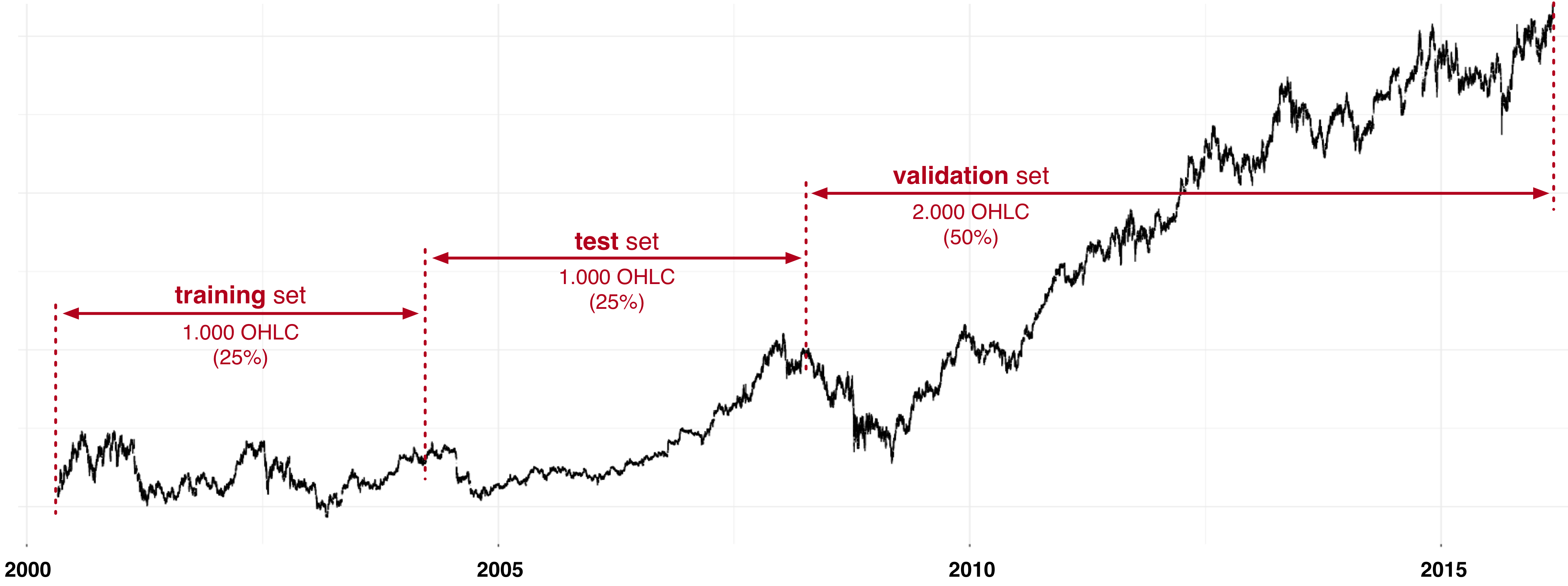
Figure 4.1: Separating data into training, test and validation set
The proposed model was initially evaluated on the shares of Apple (AAPL), Microsoft (MSFT) and Coca-Cola (KO). It yielded promising results, where it outperformed all comparative models on the test set and validation set. However, drawing conclusions based only on three sample shares may not be meaningful, so we carried out extensive testing on a larger data set and performed a confirmatory data analysis.
For the final test set we selected stocks from Russell Top 50 Index, which includes \(50\) stocks of the largest companies (based on a combination of market cap and current index membership) in the U.S. stock market. The forecasting model was tested for each stock separately. Thus, for each of the \(50\) stocks, the prediction model was trained based on past stock values of the particular stock. In the test phase, the model parameters were adjusted that the model achieved highest yield for a particular stock. The trained model with parameters tuned for the particular stock was then evaluated on validation set.
Table 4.1 shows average yield achieved by the proposed W2V model as well as yield achieved by comparative models (Buy & Hold, Moving Average (MA) and MACD) for the test and validation phase. In the test phase, average yield of the proposed W2V model was much higher than yield of the comparative models.
However, in the validation phase the results were not as good as in the test phase. The average yield of MA and MACD models were still smaller but much closer to the yield of the proposed model, while Buy and Hold outperformed our model. It still has to be noted that the proposed model achieved a positive result in all scenarios.
| Buy & Hold | MA(50,100) | MACD | W2V | |
|---|---|---|---|---|
| Test phase | $2.818,98 | $1.073,06 | -$482,04 | $11.725,25 |
| Validation phase | $16,590.83 | $6.238,43 | $395,10 | $10.324,24 |
In the test phase our model generates profit for all except one stock (i.e. JNJ), where zero profit is achieved. What is more, our model outperformed the comparative models in all but two cases (stocks SLB, JNJ). In the validation phase the results are worse but still encouraging. Only in \(14\%\) of cases the model outputs negative yield, while in \(16\%\) of cases the model outperformed all comparative models. In \(30\%\) of cases the model was the second best model. What is more, in \(7\) cases the model’s yield was very close to the yield of the best method.
In order to obtain statistically significant results we carried out Wilcoxon signed-rank test. The null hypothesis for this test is that the medians of two samples are equal (e.g. Buy & Hold vs. W2V). We accept our hypothesis for p-values which are less than \(0.05\).
| W | p-value | W | p-value | W | p-value | |
|---|---|---|---|---|---|---|
| Test phase | 2 | < 0,0001 | 1 | < 0.0001 | 1 | < 0.0001 |
| Validation phase | 427 | < 0.0210 | 155 | < 0.0001 |
Table 4.2 depicts values for test statistics \(W\) and p-values. If we focus on the test phase, obtained p-values are much lower than \(0.05\) for all three popular models. This means that there is a statistically significant difference between the resulting yields achieved by our proposed model and existing three models. For the test phase we can conclude with a high level of confidence that appropriately parametrised proposed model W2V performed better than existing three models. As mentioned earlier, the proposed model achieved slightly worse results in the validation phase.
In the validation phase the difference in returns between the proposed model and reference models was statistically significant only for MACD and MA. When compared to Buy & Hold, the W2V method yields lower returns. That can be seen already from the average yields in the Table 4.1.
The results of the proposed approach demonstrated that with the correct selection of parameters our model achieves statistically significantly better yields than the reference popular methods.
5 Conclusion and future work
Our research focused on forecasting trends in stock values. In this paper, we developed a novel approach for stock trend prediction and tested it for financial success rather than just focusing on prediction accuracy. To conduct the experiments, we selected three sample stocks – Apple (AAPL), Coca-Cola (KO) and Microsoft (MSFT) – while confirmation analysis was performed with analysis on Russell Top 50 Index.
We realized that even if the forecasting model has high prediction accuracy, it can still achieve bogus financial results, if poor trading strategy is used. A detailed analysis of the proposed forecast models in the testing phase revealed that despite the simplicity its performance was very good with statistical significance.
A more detailed analysis of trading graphs and statistical analysis showed that the proposed model has a great potential for practical use. However, it is too early to conclude that the proposed model provides a financial gain, as we have shown that selected model parameters are not equally appropriate for different time periods in terms of yield. We have also shown that the forecast model is strongly influenced by the training data set. If the model is trained with data that contains bear trend, the predictive model might be very cautious despite the general growth trend of validation data set. The problem is due to over-fitting, so training with more data would help. Some of the state-of-art machine learning algorithms like Word2Vec are dependent on a large-scale data set to become more efficient and eliminate the risk of over-fitting.
There is still room for improvement in the trading strategy. In the future, we would like to incorporate the stop loss function and already known and proven technical indicators. Future improvements also include the use of OHLC data of other stocks in the training phase as we acquire more diverse patterns that helps algorithms to detect the underlying pattern better. To improve classification accuracy and logarithmic loss, the SoftMax algorithm could also be replaced with advanced machine learning classification algorithms. One of the alternative methods of forecasting, which would be worth exploring in the future, would be a simple linear operation of aggregating vector representations of the last \(n\) Japanese candlesticks. This way we could obtain a daily, weekly or monthly trend forecast.
References
Abad, Cristina, Sten A Thore, and Joaquina Laffarga. 2004. “Fundamental Analysis of Stocks by Two-Stage DEA.” Managerial and Decision Economics 25 (5): 231–41. doi:10.1002/mde.1145.
Fama, Eugene F. 1960. “Efficient Markets Hypothesis.” PhD Thesis, Ph. D. dissertation, University of Chicago Graduate School of Business.
Fawcett, Tom. 2006. “An Introduction to ROC Analysis.” Pattern Recognition Letters 27 (8): 861–74.
Huang, Yifu, Kai Huang, Yang Wang, Hao Zhang, Jihong Guan, and Shuigeng Zhou. 2016. “Exploiting Twitter Moods to Boost Financial Trend Prediction Based on Deep Network Models.” In International Conference on Intelligent Computing, 449–60. Springer.
Jasemi, Milad, Ali M Kimiagari, and A Memariani. 2011. “A Modern Neural Network Model to Do Stock Market Timing on the Basis of the Ancient Investment Technique of Japanese Candlestick.” Expert Systems with Applications 38 (4): 3884–90. doi:10.1016/j.eswa.2010.09.049.
Kamo, Takenori, and Cihan Dagli. 2009. “Hybrid Approach to the Japanese Candlestick Method for Financial Forecasting.” Expert Systems with Applications 36 (3): 5023–30. doi:10.1016/j.eswa.2008.06.050.
Keogh, Eamonn, and Jessica Lin. 2005. “Clustering of Time-Series Subsequences Is Meaningless: Implications for Previous and Future Research.” Knowledge and Information Systems 8 (2): 154–77. doi:10.1007/s10115-004-0172-7.
Lu, Tsung-Hsun. 2014. “The Profitability of Candlestick Charting in the Taiwan Stock Market.” Pacific-Basin Finance Journal 26: 65–78. doi:10.1016/j.pacfin.2013.10.006.
Lu, Tsung-Hsun, and Yung-Ming Shiu. 2011. “Pinpoint and Synergistic Trading Strategies of Candlesticks.” International Journal of Economics and Finance 3 (1): 234.
———. 2012. “Tests for Two-Day Candlestick Patterns in the Emerging Equity Market of Taiwan.” Emerging Markets Finance and Trade 48 (sup1): 41–57. doi:10.2753/REE1540-496X4801S104.
Martiny, Karsten. 2012. “Unsupervised Discovery of Significant Candlestick Patterns for Forecasting Security Price Movements.” In KDIR, 145–50.
Mikolov, Tomas, Kai Chen, Greg Corrado, and Jeffrey Dean. 2013. “Efficient Estimation of Word Representations in Vector Space.” arXiv Preprint arXiv:1301.3781.
Mikolov, Tomas, Ilya Sutskever, Kai Chen, Greg S Corrado, and Jeff Dean. 2013. “Distributed Representations of Words and Phrases and Their Compositionality.” In Advances in Neural Information Processing Systems, 3111–9.
Mikolov, Tomas, Wen-tau Yih, and Geoffrey Zweig. 2013. “Linguistic Regularities in Continuous Space Word Representations.” In Proceedings of the 2013 Conference of the North American Chapter of the Association for Computational Linguistics: Human Language Technologies, 746–51.
Ming, Felix, Fai Wong, Zhenming Liu, and Mung Chiang. 2014. “Stock Market Prediction from WSJ: Text Mining via Sparse Matrix Factorization.” In Data Mining (ICDM), 2014 IEEE International Conference on, 430–39. IEEE.
Nassirtoussi, Arman Khadjeh, Saeed Aghabozorgi, Teh Ying Wah, and David Chek Ling Ngo. 2015. “Text Mining of News-Headlines for FOREX Market Prediction: A Multi-Layer Dimension Reduction Algorithm with Semantics and Sentiment.” Expert Systems with Applications 42 (1): 306–24. https://www.sciencedirect.com/science/article/pii/S0957417414004801.
Nison, S. 1991. Japanese Candlestick Charting Techniques: A Contemporary Guide to the Ancient Investment Techniques of the Far East. New York Institute of Finance.
Prado, Hércules A do, Edilson Ferneda, Luis CR Morais, Alfredo JB Luiz, and Eduardo Matsura. 2013. “On the Effectiveness of Candlestick Chart Analysis for the Brazilian Stock Market.” Procedia Computer Science 22: 1136–45.
Read, Jesse, Bernhard Pfahringer, Geoff Holmes, and Eibe Frank. 2011. “Classifier Chains for Multi-Label Classification.” Machine Learning 85 (3): 333.
Rousseeuw, Peter J. 1987. “Silhouettes: A Graphical Aid to the Interpretation and Validation of Cluster Analysis.” Journal of Computational and Applied Mathematics 20: 53–65.
Savić, Boris. 2016. “Tvorba Jezika Japonskih Svečnikov in Uporaba NLP Algoritma Word2Vec Za Napovedovanje Trendov Gibanja Vrednosti Delnic.” Master’s thesis, Ljubljana, Slovenia: University of Ljubljana, Faculty of Computer; Information Science. http://eprints.fri.uni-lj.si/3664/.
Shynkevich, Yauheniya, T Martin McGinnity, Sonya A Coleman, and Ammar Belatreche. 2016. “Forecasting Movements of Health-Care Stock Prices Based on Different Categories of News Articles Using Multiple Kernel Learning.” Decision Support Systems 85: 74–83.
Taylor, Mark P, and Helen Allen. 1992. “The Use of Technical Analysis in the Foreign Exchange Market.” Journal of International Money and Finance 11 (3): 304–14. doi:10.1016/0261-5606(92)90048-3.
Zhang, Dongwen, Hua Xu, Zengcai Su, and Yunfeng Xu. 2015. “Chinese Comments Sentiment Classification Based on Word2vec and SVMperf.” Expert Systems with Applications 42 (4): 1857–63. doi:10.1016/j.eswa.2014.09.011.